光デバイスのための非線形方向性結合器の数値解析

九州大学学術情報リポジトリ

Kyushu University Institutional Repository

光デバイスのための非線形方向性結合器の数値解析

前田, 洋

Graduate School of Engineering, Kyushu University

CD

NUMERICAL ANALYSIS OF

NONLINEAR DIRECTIONAL COUPLERS FOR OPTICAL DEVICES

1995

Contents

1 Introduction ₁

1.1 Backgrounds and Objective . . . . . . . . 1

1.2 Organization on the Thesis . . . 4

2 Numerical Analysis Techniques ₆

2.1 Wave Equation of Planar Waveguide . . . 6

2.2 Finite Difference Beam Propagation Method . . . 7

2.3 Definition of Normalized Transferred Power 12

3 Analysis of Two-Waveguide Nonlinear Dir~ctional Couplers 15

3.1 Introduction . . . . . . . . . . . . . . . . 15

3.2 Symmetric Nonlinear Directional Coupler with a Common Nonlinear Cou-

pling Region 18

3.3 Symmetric Nonlinear Directional Coupler with Nonlinear Waveguide Cores 32

3.4 Asymmetric Nonlinear Directional Couplers . . . . . . . . . . . 35

3.4.1 Asymmetric Nonlinear Directional Coupler with Different Wave- guide Thickness . . . . . . . . . . . . . . . . . . 35

3.4.2 Asymmetric Nonlinear Directional Coupler with Different Wave- guide Refractive Indices . . . . . . . . . . 44

3.4.3 Optical Control of Coupling Characteristics 1n Two-Waveguide Asymmetric Nonlinear Directional Coupler . . . . . . . . 50

3.5 Conclusions . . . . . . . . . . . . . . . . . . 53

4 Analysis of Three-Waveguide Nonlinear Directional Couplers 54

4.1 Introduction . . . . . . . . . . . . . . . 54

4.2 Three-Waveguide Nonlinear Directional Couplers with Identical Nonlinear Waveguide Cores . . . . . . . . . . . . 55

4.3 Optical Control of Coupling Characteristics of Identical Three-Waveguide Nonlinear Directional Coupler . . . . . . . 67

4.4 Three-Waveguide Nonlinear Directional Couplers with Nonidentical Wave- guide cores . . . . . . . . . . . . . . . . . . . . . . 69

4.5 Conclusions . . . . . . . . . . . . 78

Acknowledgment ₈₃

Bibliography 84

Glossary of Symbols Used 90

Chapter 1

Introduction

1 . 1 Backgro unds and Objective

The research on electromagnetic wave propagation in nonlinear dielectric materials has been developed to date. Electromagnetic waves in the material show interesting and widely applicable phenomena such as the optical bistability[1], the second harmonic gen- eration, solitons, and the self focusing[2]. Recently, the applications of these nonlinear effects for a optical-waveguide device come into prominence so as to realize ultra-fast all-optical-signal-processing in integrated optical circuits. The nonlinear directional cou- pler (NLDC) which makes use of the directional coupling between Kerr-like nonlinear waveguides is one of the most promising devices. The function is governed by the linear coupling of two waveguides in close proximity and its nonlinear modulation due to the change of refractive index depending on the optical field intensity. During the past several years, a symmetric NLDC structure in which two linear planar waveguides separated by a common nonlinear gap layer [3]-[10] or the reversed situation [11]-[13] has been extensively

analytical closed description of the operating characteristics of NLDC such as the critical power for switching. Various formulations of the coupled-mode analysis of NLDC are possible depending on the choice of propagation model. Jensen [3) made a significant initial effort on the coupled-mode analysis, in which the modal fields of the isolated linear waveguides were employed as the basis of propagation model and the nonlinear effect in the coupling was accounted for only by the self-phase and the cross-phase modulation terms. The difficulties and the shortcomings of Jensen's simple analysis has been recently criticized and several improvements have been reported [4)-[8). Meng and Okamoto [7) made a substantial contribution in those improvements. They employed the modal fields of the isolated nonlinear waveguides as the basis and derived the improved coupled-mode equations in which all of the coefficients depend on the optical power. Dios et al. [8) followed up the work of Meng and Okamoto [7) with a further investigation, and developed the coupled-mode analysis based on the nonlinear supermodes of the composite waveguide system. Although these new treatments yield needed improvements, it is difficult, In general, to assert the validity and the accuracy of the solutions by the method itself. It is also noted that the coupled-mode analysis by Dios et al. [8) must resort to an involved numerical calculation to obtain the nonlinear supermodes.

One of the representative numerical approaches to the NLDC to verify the analytic coupled-mode solution is the direct solution method of nonlinear differential equation using the orthogonal collocation method[l4)[15). In this method, the electromagnetic fields governing the NLDC structure are first expanded in terms of Hermite-Gaussian functions and the Helmholtz equation is transformed into a set of matrix differential equations which is solved efficiently by making use of the orthogonality of the coefficient matrix. Some important characteristics such as the coupling length and the critical power of the NLDC can be obtained also from this method (26)-[29) (37)-[39). This method

is a reliable numerical technique for various guided wave problems, which allows the numerical computation of field distributions using the step size as small as required in both directions. However, the number of collocation points is limited because of the overflow in the computation of weighted function. In this sense, the use of orthogonal collocation method is restricted to relatively small structure model.

The more accurate numerical approach to NLDC is represented by the beam- propagation method (BPM), which provides a unified treatment of various guided wave structures within the paraxial approximation. Wabnitz et al. [9] and Thylen et al. [10]

used the BPM based on the Fast-Fourier-Transform algorithm (FFT-BPM) [16] to sim- ulate the propagation of nonlinear waves in the coupler. Their numerical examples are mainly concerned with the behavior of power transfer along the waveguides. The rigorous numerical evaluation of the coupling length and critical power is of significant importance not only to verify the validity of coupled-mode approximations but also to demonstrate the precise device parameters for optical switching.

The purpose of this thesis is to develop a rigorous numerical analysis of the symmet- ric and asymmetric NLDC and to provide the highly accurate numerical results of the coupling length and critical power. The coupling nature of NLDC near the critical power changes sensitively, depending on the change of nonlinear refractive index in the propa- gating and transverse directions. Consequently, its numerical study requires a precise treatment of the nonlinear refractive index that is a function of electric field intensity.

Here we shall apply the beam propagation method based on the finite difference

pared with those of two-waveguide NLDC. We will find some important coupling charac- teristics such as the optical control, which can be applied as novel optical devices. The extension of the problem from two-waveguide couplers to three-waveguide couplers is very easily achieved in the numerical simulation than in the analytical approach.

1.2 Organization on the Thesis

This thesis is organized from five chapters. In chapter 2, the formulation of FD-BPM is explained in detail. To evaluate precisely the nonlinear refractive index change in one small propagation step size, we introduce the iteration procedure. As an index of the optical power transfer which is carried along the NLDC, the normalized transferred power is defined by using the discretized electromagnetic field.

In chapter 3, the power transfer characteristics of symmetric and asymmetric two- waveguide nonlinear directional couplers are numerically investigated in detail by FD- BPM. This method allows us to set the desired space discretization for the differenciation as fine as possible. Before starting the simulation, the discretization grid size is carefully determined. Two kinds of symmetric NLDC are first considered in the succeeding two sections. One is composed of two identical linear waveguide-cores and a common nonlin- ear cladding layer. The other is a NLDC with two identical nonlinear waveguide-cores situated in linear claddings. The numerical results for the power transfer characteristics are presented. In the third section, a novel asymmetric NLDC structure is proposed that consists of a nonlinear waveguide-core and a linear waveguide-core situated in a linear claddings. The power transfer characteristics are analyzed for two different excitation conditions; the excitation of one of two waveguides and the excitation of both waveguides with the combination of different input powers.

In chapter 4, we investigate two kinds of planar three-waveguide NLDC. One is composed of three identical nonlinear waveguide-cores in linear claddings. The other is a NLDC with two identical linear waveguides situated both sides of a center waveguide with nonlinear Kerr-like medium in linear claddings. The input/output characteristics of these three-waveguide NLDCs are analyzed numerically by FD-BPM for the linear TE₀ incident wave. We also investigate the case that the weak control light is simultaneously given into the center waveguide-core when one of the outer waveguide is illuminated by the signal light. Numerical results demonstrate that the proposed three-waveguide NLDCs are more useful for optical power filtering and switching devices than the two-waveguide NLDC.

In chapter 5, the results obtained throughout this study are briefly summarized.

Some future subjects are also mentioned.

Chapter 2

Numerical Analysis Techniques

2.1 Wave Equation of Planar Waveguide

We consider the light wave propagating in the inhomogeneous medium with refractive index n(x, y, z) and the constant permeability f-Lo· From Maxwell's equations, we can derive following Helmholtz equations which the electric vector field £ and the magnetic vector field 1i of the wave satisfies, respectively,

(2.1)

(2.2)

where

a. a. a.

\l

= ox

^'tx

⁺ oy

^'ty

⁺ oz

^{'tz, (2.3)}

and k₀ is the wave number in free space. The time dependence of the monochromatic light wave exp(jwt) is assumed and the expression is omitted throughout this thesis. In many optical waveguides, the variation of refractive index profile is very small, i.e. \l ( n ²⁾ ~ 0.

Therefore the third terms of Eq.(2.1) and Eq.(2.2) are negligible, respectively.

Generally, the configuration of many optical devices is three dimensional. The general

behavior of electromagnetic wave must be described by three-dimensional Eqs.(2.1) and (2.2). However, in most of optical devices, we can make use of the effective index method [21] and convert the three-dimensional problem to a pair of the two-dimensional (planar) one. Therefore, we are supposed to investigate the wave propagation in a planar optical device, such as a directional coupler depicted in Figure 2 .1. Practically, we can reduce the dimension of Eqs.(2.1) and (2.2) by letting

a jay=

^0.

The modes of the planar waveguide can be classified as TE(Transverse Electric) and TM(Transverse Magnetic) modes. The flow of NLDC analysis procedure for both modes is as follows. For TE mode, we choose the unique electric field of transverse direction as the leading field and calculate the value of nonlinear refractive index directly from this leading field. For TM mode, we choose the transverse magnetic field as the leading field and estimate the value of nonlinear refractive index utilizing the derivatives of the leading field which yield to a pair of electric field components. We refer to only TE mode in this thesis because the analysis of TM mode is essentially similar to that of TE mode in the analysis procedure. Using above conditions, we obtain the scalar Helmholtz equation for the transverse electric field Ey of TE mode:

(2.4) This is the starting equation of the numerical analysis of this thesis.

2.2 Finite Difference Beam Propagation Method

Ey of the TE polarization satisfies the following

/

... ... _~::

... cladding ... ...

... ...

... ...

... ...

7

< ^.or _:-,..,..~

...

~ ... X

...

L:z

... coupling ... ... ...

... ... layer ^y

... _{~ ·}

)

^~

L C y

substrate

Figure 2.1: Configuration of the planar waveguide.

where k0 and n(x, z, Ey) denote the wave number in free space and the refractive index profile, respectively. The refractive index in the Kerr-like nonlinear layer changes in proportion to the electric field intensity

JEyJ

² as follows;

(2.6)

where n1 and ^nNL are the linear refractive index and the nonlinear coefficient, respectively.

In this section the finite-difference scheme is applied directly for the paraxial wave equation. The coupling between waveguides treated in this thesis is quite weak because the waveguide cores are well separated from each other. Therefore we can assume that the propagating wave has a slowly varying amplitude profile and the rapidly changing phase factor with a phase constant {3. Applying this expression for the transverse electric field of TE wave, Ey ( x, z) is described as following form;

Ey(x, z) = E(x, z) exp( -j{3z) (2.7)

where E(x, z) is the amplitude envelope function. Substituting Eq.(2.7) into Eq.(2.5) and utilizing the fact that the term 8² E / 8z² is negligible compared with other terms, the paraxial wave equation is obtained,

(2.8) Following the scheme of finite-difference beam propagation method, the paraxial wave equation (2.8) with an arbitrary phase constant {3 is discretized as follows:

.{3EJEm 2] - -

oz

^{Em-1- 2Em ~x2}

⁺

^Em+l

(2.9)

where Xm and !:1x are the grid points and their spacing in the x direction. The unit M of grid points is taken to be an odd integer so that the center of grids coincides with that of the guiding structure. Using Crank-Nicolson's scheme [17] in the differenciation with respect to z, Eq.(2.9) can be rewritten as follows:

with

a= 2j{3

(2.11)

(2.12) (2.13) (2.14) (2.15)

where !:1z is the small step size in the z direction, and we have assumed that the nonlinear refractive index remains constant within a sufficiently small propagation length !:1z. The effect of a small change in the nonlinear refractive index on the field distribution can be taken into account by using the second-order iteration procedure as follows:

use of the initial field E~)(z),

(b) Calculate the field E;,;) ( z

+

!:1z) with bm n²(xm, IE~)(z

+

^!:1z)j2)}/2- {3²,

(c) Calculate the field E~)(z

+

!:1z) with bm n²(xm, IE~)(z

+

^!:1z)j2)}/2- {3²,

(d) Use E~)(z

+

!:1z) as the initial field for the calculation in the next step,

where the superscripts (0), (1), and (2) represent the order of the iteration, respectively.

Equation (2.11) together with the second-order iteration results in a tridiagonal sys- tern of linear equations, which can be solved efficiently by Gaussian elimination under a suitable launching condition at the input end z = 0.

The piecewisely linear tridiagonal equations can be described by a matrix form as

where

P=

X=

Q=

Px=Q

PI -1

-1 P2 -1

0

0

-1 PM-1 -1 E1(z

+ ~z) l

E2(z

+

~z)

EM(z

+

^~z)

Ql Q2

'

-1 PM

q1E1(z)

+

E2(z) E1(z)

+

q2E2(z)

+

E3(z)

EM-2(z)

+

qM-lEM-I(z)

+

EM(z) EM-I(z)

+

qMEM(z)

(2.16)

(2.17)

(2.18)

(2.19)

In the case that a directional coupler is illuminated by the eigenmode of an isolated waveguide, the wave propagates along the coupler and well confined within the core region.

The power is seldom radiated to the infinity. Therefore in the first and the last rows of Eqs.(2.17) and (2.19), we can approximate the electric fields on the outer-most grid points to be zero. However, the computation window must be set sufficiently wide so that the

(m = 1 2 · · · ' ' ' M- 1)

where

(m -_- 2 3 · · · ' ' ' M- 1) (m = 2 3 ··· M)

' ' '

(2.21)

(2.22) (2.23) (2.24) (2.25)

2.3 Definition of Normalized Transferred Power

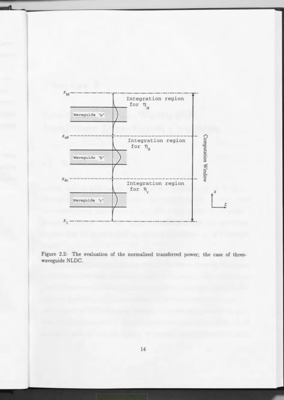
Various features of propagating waves along optical waveguides can be simulated by mak- ing use of the field distribution calculated by the numerical method given in the preceding section. For the nonlinear directional coupler which is investigated in this thesis, the eval- uation of the coupling length and the power transfer characteristics between the coupled waveguides are of most importance. For this purpose, we define the normalized transferred powers 'TJi ( z) in respective waveguides i. Figure 2.2 shows an example of three-waveguide nonlinear directional coupler. For this case, 'TJi ( z) is defined as follows;

'TJa(z) Pa(z)j ^{Pi,in, (2.26)}

'TJb(z) Pb(z)/ ^{Pi,in, (2.27)}

'TJc(z) Pc(z)/ ^{Pi,in, (2.28)}

with

Pa(z) _{_a} ^f3

[M

_{IE(x, z)j}²_dx,

2WJ-Lo Xab

(2.29)

Pb(z) - ^{f3b ["'} IE(x, z)j²dx,

2w J-Lo xbc

(2.30) Pc(z) ^{_ c f3 [ ' '} IE(x, z)j²dx,

2WJ-Lo ^x1 (2.31)

where f3a, f3b, and f3c are the linear propagation constants of each waveguide in the isolated situation. The starting and stopping points of above integrations are illustrated in Figure 2.2. x1 and XM are the outer-most sampling points located in the substrate and cover layers. Xab and Xbc are the mid-points between the waveguide a and b and between b and c, respectively. The integrations in Eqs.(2.29) to (2.31) are performed by the trapezoid formula in terms of the sampled fields Em ( z). The coupling length Lc of the coupler is given by the propagation distance z at which either TJa(z), 'TJb(z), or TJc(z) takes the first maximum depending on the launching condition at the input end z = 0.

To estimate the normalized transferred power of the two-waveguide coupler, as de- picted in Figure 3.1, the waveguide c is removed and the outer-most sampling points x₁ and xM are chosen so that they are located far enough from the waveguide in the substrate and cover region where the field intensity becomes sufficiently small.

XM - - - -

...

............ .... ... .

::::::_...waveguide _...... "a"·>:-:-:-:·:-:-: •.... , ... .

Xab - - - -

... : .. :::::.:. :-:-:-:·:-:-:-:··>>:·:··::··· I····'~···

· · ·· · · ·· ·· ··· ··· ··· I··· :v ... . ::waveguide "b":·:-:::-:::

··········

. . . . . . . . . . . . . . . . . . . . . . . .

Xbc - - - -

···················

······

::::::wa.yegu~de .. "c"::·:·::··

x,---

I· ·I ·: .. ~.~.~ .. ~.

Integration region for 11

a

Integration region for llb

Integration region for 11

c

Figure 2.2: The evaluation of the normalized transferred power; the case of three- waveguide NLDC.

Chapter 3

Analysis of Two-Waveguide

Nonlinear Directional Couplers

3.1 Introduction

Recently, there are great interests in the possibility of optical integrated devices for ultra-high-speed all-optical data processing. Two-waveguide nonlinear directional cou- plers (NLDC) are the basic elements in many of those optical circuits such as switches, dividers and combiners. The power transfer characteristics of NLDC have been widely investigated by the analytical [3]-(8] and numerical (9]-(13] techniques for a couple of decades.

The refractive index of the third-order nonlinear Kerr material shows the dependence on the electric field intensity of light wave itself. For the purpose of the control of the coupling characteristics by the optical light intensity, Jensen (3] applied the material to the coupler for the first time. Since the presentation of his theoretical work, many researchers

as the critical power for switching. Various formulations of the coupled-mode analysis of NLDC are possible depending on the choice of propagation model. Although these formulations give some predictions of the characteristics, it is difficult to assert the validity and the accuracy of the solutions by the method itself.

On the other hand, one of the representative numerical approaches to the NLDC to verify the analytic coupled-mode solution is the direct solution method of nonlinear differ- ential equation using the orthogonal collocation method [14]. This is a reliable numerical technique for various guided wave problems. However, the number of collocation points is limited because of the overflow in the computation of weighted function. In this sense, the use of orthogonal collocation method is restricted to relatively small structure model.

The more accurate numerical approach to NLDC is represented by the beam- propagation method (BPM), which provides a unified treatment of various guided wave structures within the paraxial approximation. Wabnitz et al. [9] and Thylen et al. [10]

used the BPM based on the Fast-Fourier-Transform algorithm (FFT-BPM) [16] to sim- ulate the propagation of nonlinear waves in the coupler. Their numerical examples are mainly concerned with the behavior of power transfer along the waveguides. The rigorous numerical evaluation of the coupling length and critical power is of significant importance not only to verify the validity of coupled-mode approximations but also to demonstrate the precise device parameters for optical switching.

In this chapter, the power transfer characteristics of symmetric and asyrnmetric two- waveguide nonlinear directional couplers are numerically investigated in detail by the finite difference beam propagation method (FD-BPM) [30][31]. This method allows us to set the desired space discretization for the differenciation as fine as possible. Before starting the simulation, the discretization grid size is carefully determined. Two kinds of

symmetric NLDC are first considered in the succeeding two sections. One is composed of two identical linear waveguide-cores and a common nonlinear cladding layer. The other is a NLDC with two identical nonlinear waveguide-cores situated in linear claddings. Some numerical results for the power transfer characteristics are presented using the FD-BPM.

In the fourth section, a novel asymmetric NLDC structure is proposed that consists of a nonlinear waveguide-core and a linear waveguide-core situated in linear claddings. The power transfer characteristics are analyzed for two different excitation conditions;

the excitation of one of two waveguides and the excitation of both waveguides with a combination of different input powers.

Generally in the NLDC structure, following three stages of the output characteristic are observed as a function of the input optical power level.

1. Relatively low power level

The coupling characteristics are very similar to the linear coupler because the nonlin- ear refractive index modulation is small enough. The optical wave couples perfectly from the input waveguide to the adjacent with increasing the coupling length as the input power level is increased to the critical power.

2. Critical power level

Due to the close proximity of waveguides, the input power in one waveguide is divided into another waveguide. Once the power is divided to each waveguide, the optical wave never couples anymore and propagates keeping the split state.

This input power level is referred to as a critical power. If the NLDC has two

3. Over the critical level

When the input power exceeds the critical level, the input wave couples imperfectly any longer. If the power is far over the critical, the input wave is trapped in the nonlinear region in which the refractive index is strongly modulated by the input power itself, and never couples to the adjacent waveguide.

The change of the coupling behaviour mentioned above is very important in the applica- tion for all-optical-signal-processing. We demonstrate these stages in the following chapter as results of numerical simulations.

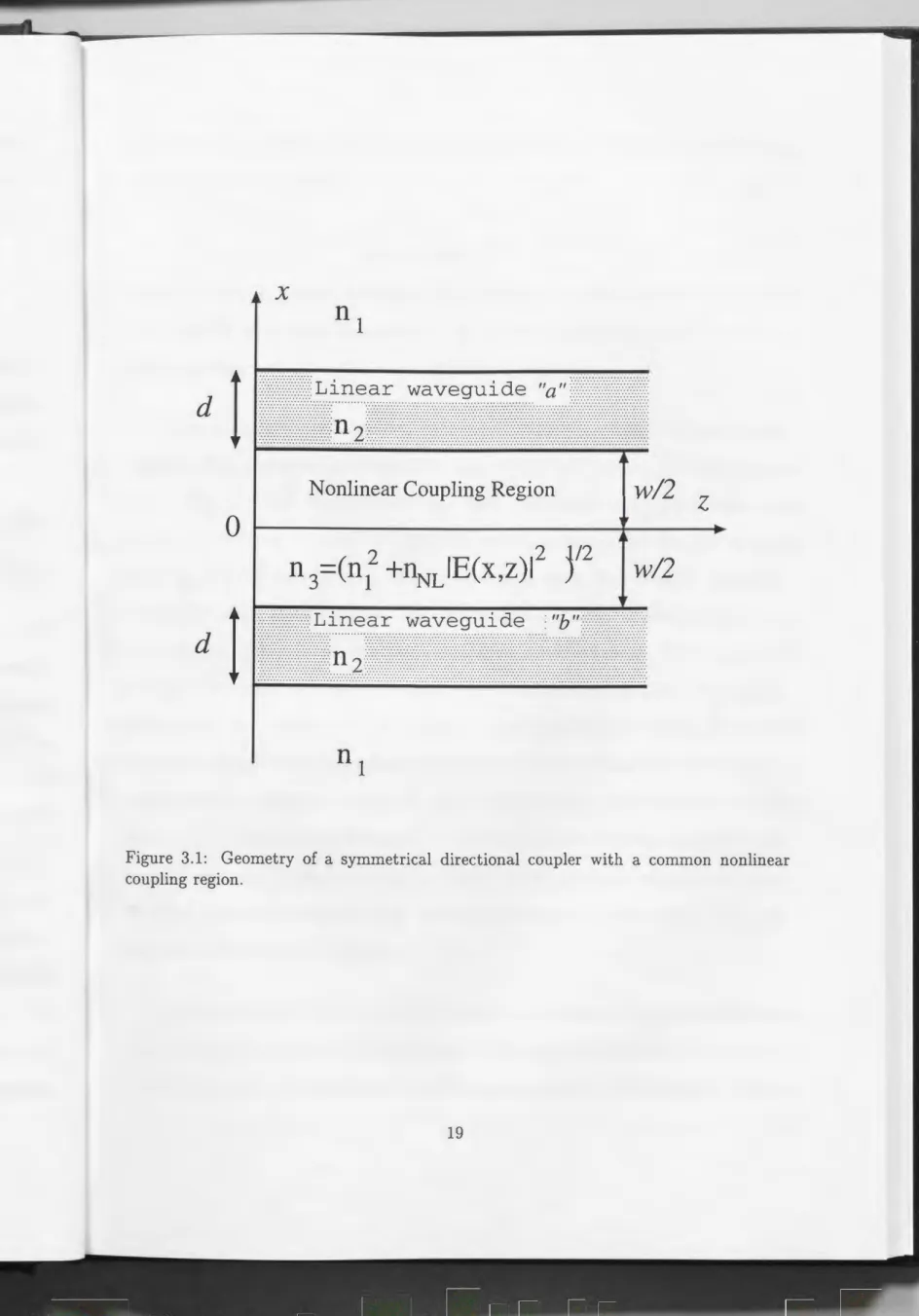
3.2 Symmetric Nonlinear Directional Coupler with a Common Nonlinear Coupling Region

The geometry of a symmetric NLDC with a common nonlinear gap layer is shown in Figure 3.1. Two identical planar waveguides a and b with a linear medium of a refractive index n2 and a width d are situated parallel to each other with a separation distance

w. The cover and substrate layers are composed of a linear medium with a refractive index n_{1 ,} and the intermediate layer of width w is of a Kerr-like nonlinear medium with a refractive index

where nN L denotes the nonlinear constant of the medium. The geometry is uniform in the y and z directions. We consider the light of wavelength ).

=

1.064 [f..Lm] and take the values of parameters for NLDC in Figure 3.1 to be n2 = 1.57, n₁ = 1.55,

nNL

=

6.377 x 10-¹² [m² /V^2], and d

=

2.0 [f..Lm]. Those values of parameters are the same as in Ref.[7]. As the initial data for Eq. (2.11), we assumed that the linear T E0 mode of waveguide a alone with nN L = 0 is incident at the input end z = 0. The amplitude of the

~~ X

nl

......

Linear waveguide

"a"

. ^~

....

^{~ .}

.... n2

·~

Nonlinear Coupling Region w/2 z

0

~

^{.. ..}

2 2

n 3=(n1 +nNL IE(x,z)l )12 _w/2

,~

..

Linear waveguide _{: "b}

^{. ..}

...

n2 .... :::

··:

n 1

Figure 3.1: Geometry of a symmetrical directional coupler with a common nonlinear coupling region.

input wave Ei,max [V/m] specified at x

=

^±(d

+

^{w)/2 and} z

=

^{0 is related to the input}

power Pi,in [W/m] as follows:

Ei,max = 2wJ..Lo

2f3od

+

f3o/ro ^Pi,in, (i = a,b) (3.2)

where w

=

27rco/ -\, c0 is the velocity of light in free space, J..Lo is the permeability in free space which is supposed to be constant in all the region, ro =

(!35 - k5ni)

¹1^2, and {3₀ is the propagation constant of the linear T E₀ mode in isolation.

Before starting the computation, we need to clarify the relation between the con- vergence of the numerical results and the small discretizing distances. We investigated the convergence of the coupling length in a linear directional coupler whose separation distance w = 2.0[J..Lm], using the FD-BPM. The other parameters used here are the same as in Figure 3.1, except that nNL = 0. For these parameters, the waveguide in isolation satisfies the single mode condition. The width of computation window is fixed to be

lxl

~ 8.0[J..Lm], while the number of grid points along x axis is variable. The waveguide a in Figure 3.1 in the linear limit is illuminated by a fundamental TE₀ mode of an isolated linear waveguide. In Figure 3.2, the coupling length is plotted as a function of a small propagation length for four typical spacing distances 6.x along x axis. The coupling length is obtained as a propagation length at which the normalized transferred power defined by Eq. (2.27) takes the first maximum. It is shown that the coupling length converges very well when 6.x ~ 0.05[J..Lm] and 6.z ~ l.O[J..Lm]. For the numerical computation by the FD-BPM, therefore, the number of grid points and their spacing were chosen as M = 321 and 6.x = 0.05[J..Lm] in the x direction.

In the numerical analysis of a NLDC, we should carefully determine the small step size along z axis considering that the electromagnetic field changes slightly and continuously in a small distance 6.z. To determine the suitable step 6.z in the z direction with or without

,---, 640 E

~

...c

+-'

~ 630

Q) _J

0>

c:

§- 620

0

0

~

(\) Q)

_s ⁶¹⁰

0.2

---

_'

\ , ,

0. 1 -- -- ---• --- --\/

^\

, ,

, ^{, •}

.. ^-

_\

. 0.025\--~

~x=0.05 ^{[ fL m]l?f \}

\

\

\

\

\

\

Figure 3.2: The linear coupling length for w = 2.0[f.1m] as a function of small propagation step size ~z for four typical spacing distance ~x.

the iteration procedure mentioned in Section 2.2, we investigated the convergency of the critical power for a NLDC in Figure 3.1 with w = 2.4(p,m]. The result is shown in Figure 3.3 as a function of small propagation step 6.z. Consequently, the second order iteration procedure provides the needed accuracy even for 6.z

=

2.0(p,m]. If we do not use the second order iteration in the FD-BPM analysis, we must set 6.z = 0.1(p,m] as a reasonable choice from the result in Figure 3.3.

When we analyze the strongly coupled NLDC which is treated in Ref. [11] with the higher refractive index, the smaller difference between core and claddings, the narrower waveguide separation, the watchful attention must be paid. In such a strongly coupling case, the iterative procedure such as Adams-Moulton formula will play an important role in the convergence of numerical solutions.

We also examined carefully the energy conservation error of the numerical solutions, and we get 6.z

=

0.5(p,m], 6.x

=

0.05(p,m] and M

=

321 with the second order iteration procedure, for which the energy conservation error less than 10-⁶ is attained.

Figure 3.4 shows the normalized transferred power TJb(z) obtained by the FD-BPM as the functions of propagation length z for w

=

3.0(p,m] and for different seven input power levels Pa,in. The propagation length z at which TJb( z) takes the first maximum gives the coupling length Lc· For Pa,in :::; 47.6[W/m], the full power transfer into the waveguide b is achieved and Lc increases with increasing Pa,in· For Pa,in

>

47.61[W/m], only a fraction of incident power is transferred and Lc decreases with increasing Pa,in· The critical power Pc for switching from waveguide b to waveguide a is numerically estimated by the incident power which yields an extremely long coupling length. We have Pc = 47.61[W/m) for the present case.

72

~ x=0.05 [ J1 m]

^X

I

I I

71

^{I I}

I I

I

r---1 _I

E

^{I I}

..._ _X

s No iteration

^{, ,}

L--...1

0

70

^,

0....

_{~ ___}

:

x-

"

"

~ 8 8 8"

i

^{8 0}

^~

69 Second order iteration

Figure 3.3: The critical power Pc as a function of 6.z for w

=

2.4[p,m]. The solid and dashed line indicate the result of second order iteration and of no iteration, respectively.

rJb 1

Linear

P a,in=20.0 , [W/m]/ 1

I

I

40.0 0.5 47.0

0 1

I

, / /

2

,

3

'

4 z[mm]

Figure 3.4: The normalized transferred power TJb as a function of the propagating distance z for w = 3.0[,um] and for different seven input power levels Pa,in·

Figures 3.5 shows the bird eyes' views of the evolutions of the normalized field dis- tribution JE(x, z)J/ Ea,max along the coupler for w = 3.0[J.Lm] and for four typical input power levels; (a) the linear case, (b) Pa,in

=

47.6l[W/m], (c) Pa,in

=

65.0[W/m], and (d) Pa,in = 80.0[W/m]. When Pa,in = 80.0[W/m] that is far above the critical power Pc = 47.6l[W/m], the incident linear TEo mode is changed into the nonlinear surface- wave mode of the waveguide a in isolation as the wave propagates. The peak of the amplitude JE(x, z)J of the nonlinear surface wave is located in the nonlinear gap layer near the core boundary of the waveguide a.

Figure 3.6 shows the coupling length Lc as a function of incident power Pa,in for w

=

2.4[J.Lm]. The results of the simple coupled-mode theory [3] and the improved coupled- mode theory [7] are also plotted for the comparison. The critical power Pc at which

Lc increases abruptly to infinity is given by 69.4[W/m], 127[W/m], and 65[W/m] for the FD-BPM, the simple coupled-mode theory, and the improved coupled-mode theory, respectively. We can see that the coupling length obtained by the improved theory [7]

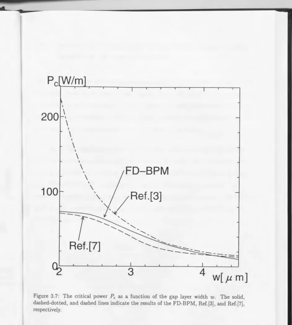
is in good agreement with that of the present numerical analysis, except for the small difference near the critical power. Figure 3. 7 shows the critical power Pc as a function of the gap layer width w, compared with the results of Ref. [3] and Ref. [7]. The critical power obtained from the improved coupled-mode theory [7] agrees well with that of the present analyses over the wide range of w, whereas the simple coupled-mode theory [3]

leads to the much larger critical power in the strongly coupling regime with w smaller than 3.0[J.Lm].

IE(x,z)I/E_a,max

0.5

0

-8.0

8.0

(a) x[micron]

z[mm]

4.0

Figure 3.5: (a) Bird eyes' views of the evolutions of normalized electric field distribution JE(x, z)J/ Ea,max along the linear directional coupler for w = 3.0[p.m).

IE(x,z)I/E_a,max

0.5

0

-8.0

8.0

(b) x[micron]

z[mm]

4.0

Figure 3.5: (b) Bird eyes' views of the evolutions of normalized electric field distribution JE(x, z)J/ Ea,max for w = 3.0[p,m] and for the input power level Pa,in = 47.6l[W/m].

IE(x,z)I/E_a,max

0.5

0

-8.0

(c)

8.0 x[micron]

0

z[mm]

4.0

Figure 3.5: (c) Bird eyes' views of the evolutions of normalized electric field distribution IE(x,

z)l/

Ea,max for w

=

3.0[J-Lm] and for the input power level Pa,in

=

65.0[W/m).

IE(x,z)I/E_a,max

0.8 0.6 0.4 0.2 0

-8.0

8.0

(d) x[micron]

z[mm]

4.0

Figure 3.5: (d) Bird eyes' views of the evolutions of normalized electric field distribution IE(x,

z)l/

^Ea,max for w = 3.0[J.Lm] and for the input power level ^Pa,in = 80.0[W/m].

O.SQ ₅₀

----

:~FD-BPM

\

\

\

\

\

1 00 Pin[W/m]

Figure 3.6: The coupling length Lc as a function of the incident power Pin for w = 2.4(J.Lm].

The solid, dashed-dotted, and dashed lines indicate the results of the FD-BPM, Ref.[3), and Ref. [7], respectively.

\

\

\

\ FD-BPM

\

100 ^\

_ \, ,/Ref.[3]

-r-....

...

,,

'

... ...

"

...

... ...

"

...

... :----...

... '::::::...

Ref. [7] --- ___ _::-:_::-- ____ _

---

4 w[ Jl m]

Figure 3. 7: The critical power Pc as a function of the gap layer width w. The solid, dashed-dotted, and dashed lines indicate the results of the FD-BPM, Ref.[3], and Ref.[7], respectively.

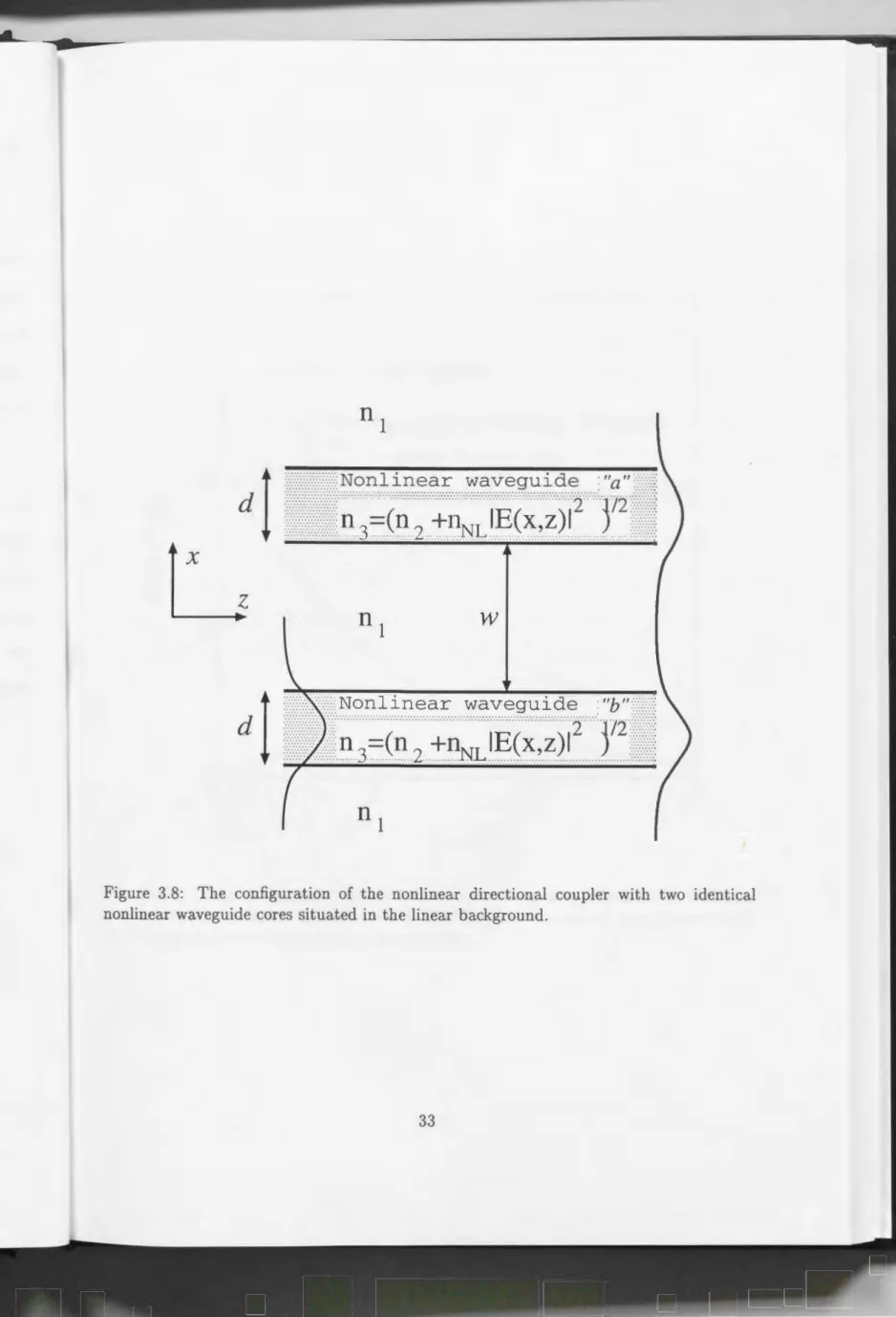
3.3 Symmetric Nonlinear Directional Coupler with Nonlinear Waveguide Cores

The other configuration of a symmetric two-waveguide NLDC is depicted in Figure 3.8.

This NLDC also provides a critical state. However, the critical power level is expected to be relatively small compared with the NLDC which was analyzed in the previous section because the refractive index of nonlinear waveguides is very strongly modulated due to the concentration of the optical field in the nonlinear waveguide core.

A set of the small step size ~x and ~z are chosen as 0.05 [JLm] and 0.1 [JLm] without the iteration procedure, respectively. The number of grid points along x axis M is 401.

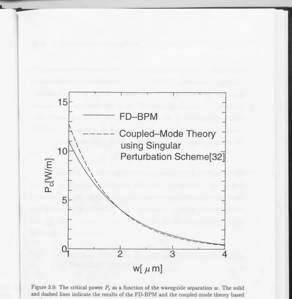
For the parameters n1 = 1.53, n₂ = 1.55, nNL = 6.38 x 10-¹²[m² /V²], d = 2.0[JLm], A

=

1.064[JLm], the critical power level is depicted in Figure 3.9 as a function of the waveguide separation w. The solid and the dashed lines indicate the result of the FD-BPM and the coupled-mode analysis using a singular perturbation scheme [32], respectively.

Both curves agree well in very wide range of w.

:::::>::::::Nonlinear waveguide

•• •••••··· ••••··~···.·.·.·.···(~···:~·.·.··· ,Ec~·,·;), ^{2 ··. · . · . ). 12} ·••••••••••••·••:

::::. -:·: ... 3 .. -... ··.·.2 ...

NL ... ... .. .

w

······

••••···~·· 3 ···c~.·.·~·.·.irl~~· '?C~.'.i).I

²

··•· ^{· ; 12}

Figure 3.8: The configuration of the nonlinear directional coupler with two identical nonlinear waveguide cores situated in the linear background.

10

5

FD-BPM

- - - Coupled-Mode Theory using Singular

Perturbation Scheme[32

2 3 4

Figure 3.9: The critical power Pc as a function of the waveguide separation w. The solid and dashed lines indicate the results of the FD-BPM and the coupled-mode theory based on the singular perturbation scheme, respectively.

3.4 Asymmetric Nonlinear Directional Couplers

Two-waveguide asymmetric nonlinear directional couplers, which have a nonlinear and a linear waveguide core, are numerically analyzed by FD-BPM in this section. These NLDCs are designed so as to be the phase-mismatch state in the low input power level. As the input optical power increases, the phase of two waveguides matches due to the optical refractive index modulation of the nonlinear Kerr material and the perfect power transfer between two waveguides is attained at a suitable power level. This power-dependent coupling characteristic is applicable for an optical switch or an optical power filter [27]- [31].

It is possible to realize the asymmetry of the coupler by two means ; one is to change the linear part of refractive index of each waveguide core and the other is to change the thickness of each one. At first, we analyze the asymmetric nonlinear directional coupler with different waveguide thickness. Next, the asymmetric nonlinear directional coupler with different waveguide refractive index is analyzed. Several power dependent coupling phenomena are observed [ 31].

3.4 .1 Asymmetric Nonlinear Dir e ctional Coupler with Differ- ent Waveguide Thickness

The side view of an asymmetric NLDC is shown in Figure 3.10. A linear waveguide a of width 2da and a nonlinear waveguide b of width 2db are situated parallel to each other with a separation distance w. The refractive index of the core of linear waveguide a is n2

X

w/2 z

0

w/2

·:::::::::::Nonlinear waveguide ·

''b'' :::::::::::··

···~4···c?; ··· ;?~·~··IE(~,~·)·12 .·.·.·· ^{)12 ...}

Figure 3.10: Side view of an asymmetric nonlinear directional coupler composed of a linear waveguide a and a nonlinear waveguide b.

the same expression as what we treated in the previous sections, with a refractive index

(3.3)

where n3 and nNL denote the linear refractive index and the nonlinear coefficient of the medium, and IE(x, z)l² is the intensity of electric field. The geometry is uniform in the y and z directions. We examine the propagation of a two dimensional TE wave. The behaviour of the transverse electric field amplitude E is described by Eq.(2.8). Under the paraxial approximation, we can obtain the same finite difference formulation as Eq.

(2.11).

The fixed parameters used throughout this section are the wavelength .A = l.O[J.Lm], the nonlinear coefficient nN L

=

6.377 x 10-¹² [m²

/V

^{2], and the linear} refractive index n1 == 1.53, which is common in the cladding, gap, and substrate layers. As the initial data for Eq.(2.11), we assumed that the linear TE0 mode of the isolated waveguide a orb is incident into the waveguide a or the waveguide b of the NLDC at the input end z

=

0, respectively. When the initial launching condition is specified, the amplitude ^Emax of the incident TE0 mode defined at the core center x = w

+

^da or x = -w -db is related to the input power Pi,in as follows:

Emax = ( i

=

^a or b), (3.4)

where w and J.Lo are the angular frequency of light and the permeability in free space,

ri =

J

^{{3[ -}

^k6ni,

^{and f3i} is the propagation constant of the linear TE₀ mode of waveguide i. For the numerical computation, we have taken the reference wavenumber {3 in Eq.(2.11) to be (f3a

+

f3b) /2, and chosen the computation area in the x direction, the number of grid

chosen as 6z

=

0.1 [J.Lm] without the iteration, after having confirmed that the error in power conservation with propagation remains less than 10-⁶ over the propagation length 0

<

z::::; 2[mm].

We consider first the case in which the two cores of NLDC have the same refractive index in the linear limit but different widths. Figure 3.11 shows the normalized transferred power 'TJa(z) = Pa(z)l Pa,in in the linear waveguide a defined by Eq.(2.26) as functions of propagation length z for da = 2.2[J.Lm], db = 2.0[J.Lm], w = 2.0[J.Lm], n2 = 1.55, and for different several input power levels Pain ) launched into the linear waveguide a. In the linear limit with nNL

=

0 or _{n 3}

=

n 2 , only a fraction of input power is transferred between the two waveguides. The rate of power transfer increases with the increment of input power, and a nearly complete power transfer into the waveguide b is attained when Pa,in

=

4.0[Wim]. For further increase of input power, the rate of power transfer is decreased rapidly. The propagation length for the complete power transfer is estimated as z = l.O[mm], which is about twice the coupling length in the linear limit. Figure 3.12 shows the normalized transferred power 'TJa ( z)

=

Pa ( z)

I

^Pb,in as functions of propagation length z for different several input power levels Pb,in initially launched into the nonlinear waveguide b with the same parameters as in Figure 3.11. For the input power around Pb,in = 4.0[Wim], nearly complete power transfer from the waveguide b to the waveguide a is obtained at the propagation length z = l.O[mm], which is also about twice the coupling length in linear limit. Taking into account the features of power transfer depicted in Figures 3.11 and 3.12, we assumed the device length of NLDC to be l.O[mm] and set the output end in the linear waveguide a. Figure 3.13 shows the normalized output power 'TJa,out

=

Pa (z)

I

^{Pa,in at z}

=

l.O[mm] as a function of the input power Pa,in launched into the linear waveguide a with the same parameters as in Figure 3.11. It can be seen that the output power is strongly suppressed for the input optical signal with the power level

around 3.8[W/m]. Figure 3.14 shows the normalized output power TJa,out

=

Pa(z)/ Pb,in at the same output end as a function of the input power Pb,in launched into the nonlinear waveguide b with the same parameters as in Figure 3.11. In this case, a full output is obtained only for the input optical signal with the power level around 3.8[W/m]. When the output end of NLDC is set in the nonlinear waveguide b, we have the input/output characteristics opposite to those depicted in Figures 3.13 and 3.14 because the energy conservation is well satisfied in the present numerical computation.

1Ja

0.5

0

I I

I I I

,

I

~~ I

I #

1 /

I #

\ I

___ ...

^~ f/

p -4 0

~

a in- ·

I '

[W/m]

w=2.0[ J1 m]

1 2

z[mm]

Figure 3.11: Normalized transferred power 'TJa in the linear waveguide a as functions of the propagating distance z for da = 2.2[p,m], db = 2.0[p,m], w = 2.0[p,m], and n₂ = n3 = 1.55, and for several different input power levels Pa,in launched into the linear waveguide a.

/

..

w=2.0[ J1. m]

1^{# ' ,}

I

' \

'Ia

'

^\

'

\ 3.0

~

'

\

'

0.5

^\ _'

\

'

\

0 1 2

z[mm]

Figure 3.12: Normalized transferred power TJa as functions of the propagating distance z

for different several input power levels Pb,in launched into the nonlinear waveguide b. The values of parameters are the same as in Figure 3.11.

7J

a,out

0.5

0 5

z=1.0[mm]

w=2.0[ J1. ^m]

10 15

Pa in[W/m]

'

Figure 3.13: Normalized output power TJa,out at z = l.O(mm] as a function of input power

Pa,in launched into the linear waveguide a. The values of the parameters are the same as in Figure 3.11.

1J

a,out

0.5

0 5

z=1.0[mm]

w=2.0[ J1 m]

10 15

Pb in[W/m]

'

Figure 3.14: Normalized output power TJa,out at z = l.O[mm] as a function of input power

Pb,in launched into the linear waveguide b. The values of the parameters are the same as in Figure 3 .11.

3.4.2 Asymmetric Nonlinear Directional Coupler with Differ- ent Waveguide Refractive Indices

We consider next the asymmetric NLDC in which the two cores of NLDC have a same width but different refractive indices in the linear limit. Figure 3.15 shows the normalized transferred power TJa(z) for da =db= 2.0[J.Lm], w

=

2.4(J.Lm], n2

=

1.551, n₃

=

1.550, and for different several input power levels Pa,in· A complete power transfer to the nonlinear waveguide b is expected to occur at the propagation length around z = 2.0[mm] for a proper input power level within 5.0[W/m] < Pa,in < 6.0[W/m]. This propagation length is nearly four times as large as the coupling length in the linear limit. Figure 3.16 shows the similar results when the input power Pb,in is launched into the nonlinear waveguide b. It can be seen that nearly complete power transfer to the linear waveguide a is attained at around z ⁼ 2.0(mm] for the input power level slightly less than 4.0[W/m].

For this configuration of NLDC, therefore, we assumed the device length of 2.0[mm] and set the output end in the linear waveguide a. The input/ output power characteristics are shown in Figure 3.17 for the input into the linear waveguide a and in Figure 3.18 for the input into the nonlinear waveguide b. Compared with Figures 3.13 and 3.14, the input/output characteristics in the main response become much sharper, but on the other side, a stringent adjustment of device length is required to realize a complete power transfer between the two waveguides.

From the input/ output characteristics discussed above, it can be seen that the asym- metric NLDC in Figure 3.11 is useful for constructing a power band-pass filter or a power band-reject filter, by setting properly the input and output ends and the device length.

Before concluding, it is worth to mention the effect of the waveguide separation w on the power transfer characteristics. When the values of other parameters are fixed, there

exists an optimum separation distance for which the complete power transfer for filtering is obtained within a propagation length less than a few millimeters. As the separation distance increases, it becomes rather difficult to achieve the phase-matching between two waveguides within a realistic propagation length, the rate of maximum power transfer is remarkably reduced, and eventually the power filtering function of NLDC is diminished.

1Ja

#

I

#

I

#

0.5

10.0

I

#

, I

\

I

\ , I

\..."

, , I , I

'

,_, ,

I

P a in=6.0[W/m]

w=2.4[ J1 m] '

0 1 2 3

z[mm]

Figure 3.15: Normalized transferred power TJa as functions of the propagating distance z for da = db = 2.0[p,m], w = 2.4[p,m], n2 = 1.551, n3 = 1.550, and for different several input power levels Pa,in launched in the linear waveguide a.

rJa

0.5

0 1 2 3

z[mm]

Figure 3.16: Normalized transferred power 'Tla as functions of the propagating distance z for several different input power levels Pb,in launched into the nonlinear waveguide b. The values of parameters are the same as in Figure 3.15.

1J

a,out

0.5

0 5

z=2.0[mm]

W=2.4[ J1 m]

10 15

Pa in[W/m]

'

Figure 3.17: Normalized output power TJa,ov.t at z

=

2.0[mm] as a function of input power

Pa,in· The values of parameters are the same as in Figure 3.15.

1J

a,out

0.5

0 ₅

z=2.0[mm]

w=2.4[ J1 m]

10 15

Pb in[W/m]

'

Figure 3.18: Normalized output power TJa,out at z

=

2.0[mm] as a function of input power

Pb,in· The values of parameters are the same as in Figure 3.15.

3.4.3 Optical Control of Coupling Characteristics In Two- Waveguide Asymmetric Nonlinear Directional Coupler

We consider the case that the two waveguides of an asymmetric nonlinear directional coupler are illuminated simultaneously by the each TE₀ mode of isolated situation in the linear limit. The NLDC structure is same as shown in Figure 3.10. The asymmetry is achieved by the difference between the core thicknesses, where da = db

+

^0.2[p,m] = 2.2[p,m]. The other parameters used are the same as Section 3.4.1.

Firstly, in Figure 3.19, the bird eyes' view of the electric field intensity of propagating wave without control light is plotted. The input power in the waveguide a is Pa,in =

2.38[W/m]. It is clearly shown that the input wave couples imperfectly to the adjacent nonlinear waveguide. Under this situation, the power transfer characteristics can be drastically changed by launching additional small input power into waveguide b. Figure 3.20 shows the result for Pa,in

=

2.38[W/m] and Pb,in

=

0.40[W/m]. We can see that this combination of input power excites the nonlinear eigenmode of the NLDC and there occurs no power transfer between the element waveguides. This result suggests that we can control the power coupling between two waveguides using an additional light beam with relatively small amount of power, and is of particular importance in the application of optical switching by making use of control light.

IE(x,z) I [a.u.]

1

0.5

0

4000 -10

z[rnicron]

10 x[rnicron]

Figure 3.19: Bird eyes' view of the electric field intensity without control light. The input power of signal light Pa,in = 2.38 [W/m].