Kyushu University Institutional Repository

(1)

九州大学学術情報リポジトリ

Kyushu University Institutional Repository

大規模構造体を調査するための宇宙線ミューオン透視システムの開発

中居, 勇樹

https://doi.org/10.15017/4059988

出版情報：Kyushu University, 2019, 博士（理学）, 課程博士バージョン：

権利関係：

(2)

Development of a muography system to survey large scale structures

Yuki Nakai Kyushu University

February 27, 2020

(3)

(4)

Abstract

The muon, which is one of the elementary particles, is classified as second-generation charged lepton. Although its mean lifetime is short, approximately 2.2 µs, it rains on the ground as secondary cosmic rays at the rate of ∼1 per cm² per minute. Its mass is 105.6 MeV/c², which is approximately 200 times larger than that of the electrons. The large mass results in low energy loss upon passing through materials. Consequently, it has a stronger penetrating power than both β-rays and X-rays do. On the basis of the aforementioned features of the muon, a technique known as “muography” has been developed. Muography can be used to see through large structures by measuring the cosmic ray muons that pass through these structures, as the permeability of muons corresponds to the area density. Using this new technique, one can obtain the area-density distribution by measuring the incident angles of the muons. Moreover, this technique enables the surveying of structures in a non-destructive way. Therefore, recently, muography has been globally used to survey various large structures.

In the domain of muography, nuclear emulsion detector, gaseous detector, and plastic scintillation detectors are used to detect the tracks of muons. Although emulsion and gaseous detectors have excellent angular resolutions, an exclusive readout system and a gas circulation system are indispensable. However, although plastic scintillation detectors have poor resolutions, they are convenient to use, thereby ensuring long-term and stable operation.

Conventional photosensors, which are attached to scintillators, have certain disadvantages.

We countered these disadvantages by using new semiconductive photosensors known as silicon photomultiplier (SiPM).

We developed a muography system using 144 plastic scintillators and 288 SiPMs. This detector measures muon tracks and can reconstruct their incident angles with a resolution of 0.46^◦. Using this detector, we can measure the muon tracks and reconstruct their incident angles with a resolution of 0.46^◦. In terms of performance, the number of detected photons is 29 ± 6 photons/SiPM. The time of flight, i.e., 6.1 ns, which corresponds to the velocity of light and a detector length of 183 cm, is measured with a resolution of 1.0 ns. This resolution enables us to determine the incident direction. Consequently, with a significance of 6 standard deviations, the backgrounds due to muons from the back direction are excluded. To operate the system outdoors, we also developed an environmental monitor system and a power system. The muography system will be subjected to several temperature diﬀerences in such environments.

The monitor system records temperature at 288 points with a resolution of 0.1 ^◦C to correct the gain of the SiPMs, whose temperature dependence is 1.8%/^◦C. Because the measured temperatures can be used to correct the dependence, the SiPMs are operable outdoors. The power system comprises 1200-W solar panels, a 22-kWh power storage device, and a 3-kW emergency engine generator. Because of the power system, we can also operate the muography system without an external power supply.

On the basis of a Monte-Carlo (MC) simulation program, we established an analysis method.

The MC simulation can reproduce the response of the scintillators and the cosmic ray flux. To reject background events, the analysis method utilizes likelihood functions generated using the MC simulation program. This analysis can exclude background particles and retain muons with an eﬃciency of approximately 70%.

Using the muography system and the analysis method, we performed three measurements.

The first measurement was performed on the buildings on Ito campus, Kyushu University, and we successfully measured the area densities ofO(10³) g/cm². The second one was performed on the mountains located to the north of the campus. We observed the measured area density to be proportional to the path length of the penetrating muons. However, the measured densities were

(5)

considerably low, approximately 1 g/cm³, as background events disturbed the measurement.

The result suggests that the distance between the object and the system is critical to suppressing such backgrounds. Therefore, for the third measurement, we measured an ancient tomb, Ikenoura-Kofun. We successfully measured the area densities of O(10³–10⁴) g/cm² because of the short distance of ∼100 m.

From the results, it is evident that the system can measure an area density of at least O(10³–10⁴) g/cm². Assuming the aforementioned performance, we can use the system for scientific research. As an instance, an application of this system to measure volcanoes, called scoria cones, is possible. Aso-Komezuka, which is one of the most famous scoria cones in Japan, is an interesting target. We estimated the number of penetrating muons at some candidate locations there and showed that the internal structure of this scoria cone could be observed within approximately two weeks.

(6)

(7)

List of Figures

1.1 Energy spectrum of primary cosmic rays . . . 13

1.2 Mass stopping power for positive muons incident on copper . . . 15

1.3 Overview of the scattering method . . . 16

1.4 Overview of the absorption method . . . 16

1.5 Relation between the relative muon intensity and object thickness . . . 16

1.6 Example of the mis-reconstruction due to accidental hits . . . 18

1.7 Simulation results of the background study . . . 19

2.1 Overview of the muography system . . . 20

2.2 Detector overview . . . 21

2.3 Picture of the housing . . . 22

2.4 Overview of the NIM EASIROC module . . . 23

2.5 Overview of the information recorded by the module . . . 23

2.6 Picture of the logic board . . . 24

2.7 Overview of the monitor system and its pictures . . . 24

2.8 Display during a data-acquisition instance . . . 25

2.9 Result of the power-generation test. . . 26

3.1 (a) Correlations between HG ADC and LG ADC and (b) between LG ADC and combined ADC . . . 28

3.2 Histogram of the combined ADC . . . 28

3.3 Pedestal subtracted ADC distribution . . . 29

3.4 Histogram of the photon yields . . . 30

3.5 Example of the hit-position dependence . . . 31

3.6 Temperature dependence of an SiPM . . . 31

3.7 Histograms of the ADC and the energy deposit on the scintillator . . . 32

3.8 Histogram of the energy resolutions . . . 33

3.9 Distribution of the reconstructed energy deposit . . . 33

3.10 Hit-position dependence of the TDC . . . 34

3.11 Outline of the time walk correction . . . 35

3.12 Result of the time walk correction . . . 35

3.13 Distribution of the timing resolutions . . . 36

3.14 Definition of the axes and the incident angles . . . 37

3.15 Distribution of the reconstructed TOF . . . 38

3.16 Correlation between the hit position and the time diﬀerence . . . 39

3.17 Distribution of the position resolutions reconstructed using the time diﬀerence . 40 4.1 Detector geometry (side view) . . . 41

4.2 Detector geometry (front view) . . . 41

4.3 Calculated muon flux as a function of the zenith angle and muon energy . . . . 43

4.4 Flux distribution of electrons . . . 44

(11)

4.5 Flux distribution of positrons . . . 44

4.6 Flux distribution of protons . . . 44

4.7 Light-yield response to protons . . . 45

4.8 Comparison of the hit times between MC and data . . . 46

4.9 Comparison of the total energy deposits between MC and data . . . 46

4.10 Distributions of the total energy deposit versus TOF . . . 47

4.11 Steps to estimate the number of penetrating muons. . . 48

5.1 Distribution of TOF and χ²_T . . . 51

5.2 Distribution of ∆θ_X and χ²_X . . . 52

5.3 Distribution of ∆θ_Y and χ²_Y . . . 53

5.4 Energy deposit per 2-cm of each module . . . 54

5.5 Distribution of the likelihood ratio . . . 56

5.6 Survival probability ratio of the likelihood analysis to that of the preselection . . 56

5.7 Eﬃciency of the analysis for electrons . . . 57

5.8 Eﬃciency of the analysis for protons . . . 57

5.9 Eﬃciency of the analysis for muons . . . 57

5.10 Relation between zenith angle, ratio, and cutoﬀ energy . . . 58

5.11 Relation between cutoﬀ energy and area density . . . 59

6.1 A bird’s eye view of the buildings . . . 60

6.2 Number of detected muon-like particles in the measurements of buildings . . . . 61

6.3 Area-density distribution of the buildings . . . 62

6.4 Map of the measurement place and mountains . . . 63

6.5 Estimated path-length distribution of muons that penetrate the mountains . . . 63

6.6 Number of detected muon-like particles in the measurement of the mountains . . 64

6.7 Comparison between data and MC in the measurement of the mountains . . . . 65

6.8 Area-density distribution of the mountains . . . 66

6.9 Density distribution of the mountains . . . 66

6.10 Histogram of the measured densities of the mountains . . . 67

6.11 Bird’s eye view and corresponding map of Ikenoura-Kofun . . . 67

6.12 Picture of the Ikenoura-kofun from the rear of the system . . . 68

6.13 Number of detected muons in the measurement of Ikenoura-Kofun . . . 69

6.14 Measured area density of Ikenoura-Kofun . . . 69

6.15 Background events estimated via MC simulation in the measurement of Ikenoura-Kofun . . . 70

6.16 Estimated background events by MC in the measurement of Ikenoura-Kofun . . 70

6.17 Corrected area-density distribution of Ikenoura-Kofun after the background subtraction . . . 71

6.18 Density distribution of Ikenoura-Kofun . . . 71

6.19 Histogram of the densities of Ikenoura-Kofun . . . 72

6.20 Energy-deposit distribution of each scintillator after the path-length correction . 73 6.21 Histogram of the most probable values . . . 73

6.22 Measured area density in tanθ_Y = 0.128−0.156 . . . 75

7.1 Four major stages of the development of scoria cones . . . 77

7.2 Overview of Aso-Komezuka . . . 79

7.3 Result of the electric-resistance method . . . 80

7.4 Result of the magnetic anomaly method . . . 80

7.5 Map of the candidates for the measurement of Aso-Komezuka . . . 81

(12)

7.6 Simulation results . . . 82

7.7 Path length of the dense region with the view at SE . . . 82

7.8 Hit-rate distributions with the dense region and view at SE . . . 83

7.9 Comparison of the hit rate . . . 83

A.1 The measured area density in tanθ_Y = 0.099−0.128. . . 85

(13)

List of Tables

1.1 Basic properties of muon . . . 12

1.2 Variables used in the Bethe-Broch equation. . . 14

2.1 Detail of the power consumption of the muography system. . . 26

6.1 Systematic uncertainty of muon permeability . . . 74

(14)

Chapter 1 Introduction

1.1 Overview of this thesis

This thesis describes the development of a muography system for large-scale structures. The first chapter provides an introduction to muography. Here, we explain the principle, detectors, and background events of muography. The second chapter presents the developed muography system, and also presents the detailed design of the system. In Chapter 3, we explain the reconstruction methods to correct the measured values. The obtained performance after the correction is also shown therein. We developed two simulation programs. One simulates cosmic ray events, including the detector response, and the other estimates the number of muons that penetrate an object. The development of both the programs is shown in the next chapter. On the basis of cosmic ray simulation, we established an analysis method that utilizes likelihood functions. We describe the method in Chapter 5. Using the muography system and the analysis method, we performed three measurements, whose results are shown in Chapter 6. On the basis of the results of the measurements, we will discuss the application of the system in Chapter 7.

In the last chapter, we conclude this thesis.

1.2 Overview of muography

Recently, a new technique, called “muography”, has been developed for seeing through large-scale objects such as buildings and mountains. Muography uses elementary particles called “muons” (represented asµ). In nature, muons rain as secondary cosmic ray particles, on the ground from the sky. Measuring the permeability of muons that pass through an object, we can obtain the object density in a manner similar to that in X-ray radiography. Upon measuring the incident angles of the muons, a density distribution is reconstructed. Because muography enables us to non-destructively obtain a two-dimensional distribution of large structures, it is a powerful technique.

Historically, muography originated from the measurement performed by an Australian physicist, Eric George. He measured the depth of the overburden of a tunnel by using a Geiger-Muller counter in the 1950s [1]. Although via the measurement, he could not image the density structure because of the limitation of instruments at that time, it was the first muon-transmission application for density measurements. In 1967, Alvarez and his colleagues searched for hidden chambers in the Pyramid of Giza, Egypt [2]. Theirs was the first imaging measurement of muography, which demonstrated the feasibility of muography imaging.

Subsequently, muography has been applied in various domains, such as non-destructive surveys of a castle [3], blast furnaces [4], caves [5], pyramids [6], and volcanoes [7, 8]. Notably, the applications for active volcanoes is the most popular one, because they can be real-time

(15)

monitored. The magma dynamics in an erupting volcano was indeed observed with muography [9].

1.3 Muon and cosmic rays

Muon is categorized into the second generation of the lepton family. Table 1.1 lists the basic properties of the muon. A muon decays with a mean lifetime of ∼2.2 µs via Michel decay,

µ⁺ → e⁺+ ¯ν_µ+ν_e, (1.1)

µ⁻ → e⁻+ν_µ+ ¯ν_e, (1.2)

where ν_e (ν_µ) denotes an electron neutrino (a µ neutrino), and the one with a bar denotes an anti-neutrino. The mass of a muon is approximately 200 times larger than that of an electron, while the electric charge is the same for both of them.

Property Value

Electric charge 1.6021766208×10⁻¹⁹ C Lifetime 2.1969811 µs

Mass 105.6583745 MeV/c² Table 1.1: Basic properties of muon [10].

As primary cosmic rays, many kinds of particles arrive from the outer space into the atmosphere, and Fig. 1.1 depicts their energy spectrum. The particles interact with the atoms in the atmosphere and, consequently, produce secondary cosmic rays. A pion (π^±), which is generated by the aforementioned interaction, immediately decays into a muon with a mean lifetime of 26 ns via the following reactions:

π⁺ → µ⁺+ν_µ, (1.3)

π⁻ → µ⁻+ ¯ν_µ. (1.4)

Cosmic ray muons have high energy, because high-energy primary particles distribute their energy to the decay products including pions.

The muon flux depends on the zenith angle,θ, which is approximately described as∝cos²θ.

The energy of cosmic ray muons also depends on the zenith angle. The muons from the zenith tend to have low energy, because their parent pions interacted with considerable number of atoms in the dense atmosphere. Consequently, they distribute their energies among their daughter particles. However, the muons from the horizon tend to have high energy because their parent pions interacted with fewer atoms in a thinner atmosphere, and, therefore, the number of daughter particles decreases. Consequently, the energy per muon increases. Despite their short lifetime, the relativistic eﬀect enables cosmic ray muons to reach the surface of the earth. Muography uses the cosmic ray muons that reach the surface.

1.4 Interactions of charged particles in material

Energy loss

When relativistic charged particles pass through a material, they interact with the material via the Coulomb interaction and lose their energy via the interaction. The mean energy-loss rate,

(16)

Figure 1.1: Energy spectrum of primary cosmic rays [10].

(17)

⟨dE/dx⟩, is described using the Bethe formula [11] as follows:

⟨dE dx

⟩

=Kz²Z A

1 β²

[1

2ln2m_ec²β²γ²W_max

I² −β²− δ(βγ) 2

]

, (1.5)

wherecdenotes the speed of light in vacuum,β the relativistic velocity of the incident particle, γ the Lorentz factor defined asγ ≡1/√

1−β², andWmaxthe maximum energy transfer defined as

W_max≡ 2m_ec²β²γ²

1 + 2γm_e/M + (m_e/M)², (1.6)

and the others variables are listed in Table 1.2. Figure 1.2 depicts the mass stopping power,

⟨dE/dx⟩, for positive muons incident on copper as a function of βγ = p/M c. Practically, most relativistic particles, e.g., cosmic ray muons, have mean energy-loss rates close to the minimum. Such particles are called “minimum-ionizing particles (MIPs).” The large mass brings low energy loss to muons, thereby resulting in the strong penetrating power.

Symbol Definition Value or units

m_e electron mass MeV/c²

h Planck constant

ℏ ℏ≡h/2π

ϵ₀ the permittivity of free space

r_e classical electron radius e²/4πϵ₀ℏc

N_A Avogadro’s number

K Coeﬃcient for dE/dx 4πN_Ar_e²m_ec²

z charge number of incident particle

Z atomic number of absorber

A atomic mass of absorber

I mean excitation energy eV

δ(βγ) density eﬀect correction to ionization energy loss Table 1.2: Variables used in the Bethe-Broch equation.

Multiple scattering

When charged particles pass through a medium, they scatter along diﬀerent directions.

Most deflection is attributed to the Coulomb scattering from nuclei, as described by the Rutherford scattering. For many small-angle scatterings, the net scattering angle distributions are Gaussian-like. The scattering angle distribution due to the multiple scattering is well-represented by the theory of Moli`ere [12]. We define the net scattering angle as the root mean square of the gaussian as follows:

θ₀ =θ^rms_plane= 1

√2θ_space^rms . (1.7)

Accordingly, it is described as follows [13]:

θ₀ = 13.6 MeV βcp z

√ x X0

[

1 + 0.088 log₁₀ ( xz²

X0β² )]

, (1.8)

where p denotes the momentum of the incident particle, X₀ the radiation length¹, and x the thickness of the medium. The other parameters are the same as those in Table 1.2.

1The length at which the energy of the incident electron traversing the medium becomes 1/e.

(18)

Muon momentum

1 10 100

Mass stopping power [MeV cm2/g] Lindhard- Scharff

Bethe Radiative

Radiative effects reach 1%

Without δ Radiative

losses

0.001 0.01 0.1 1 10 βγ 100

100 10

1 0.1

1000 10⁴ 10⁵

[MeV/c]

100 10

1

[GeV/c]

100 10

1

[TeV/c]

Minimum ionization

Eµc

Nuclear losses

µ⁻

µ⁺on Cu

Anderson- Ziegler

Figure 1.2: Mass stopping power for positive muons incident on copper [10].

1.5 Principle of muography

In muography, the following two types of methods exist: the scattering method and the absorption method. We describe their principles and overviews here.

1.5.1 Scattering method

The scattering method provides density information by measuring scattering positions and angles. Figure 1.3 depicts an overview of the scattering method. This method needs two tracks of a muon both before and after passing through the object. The intersection of both the tracks corresponds to the position of the object, and the deflection angle reflects its density, as described in Eq. (1.8) and the Rutherford scattering. This method utilizes vertically incident cosmic ray muons to collect suﬃcient data. Consequently, the scattering method is suitable to scan the object in a short time.

However, two detectors with a fine angle resolution are indispensable for this method. The scattering method is not usable for such as mountains because we cannot cover such large-scale objects by using detectors. Therefore, this method is applied to small-scale structures at most several meters. For instance, scan systems for containers with the scattering method have been installed in some ports by a commercial company [14].

1.5.2 Absorption method

The absorption method measures the flux and incident angles of cosmic ray muons. Figure 1.4 depicts the overview of the absorption method. A thick object shields low-energy muons because of the energy loss in materials [see Eq. (1.6)]. Therefore, the survival rate of cosmic ray muons corresponds to the object thickness. Figure 1.5 depicts a relation between the relative muon intensity and object thickness. On the basis of the relation, we can convert the permeability of the muons into the object thickness. Generally, the absorption method utilizes horizontally incident muons for massive objects. Because the flux of horizontal muons is small, long-term

(19)

Detector (1)

Detector (2)

Reconstruct the position from the tracks

Estimate the density from the deflection angle Muon track

Figure 1.3: Overview of the scattering method.

Cosmic ray muons (well-known)

Detector (measure)

Object (unknown)

Figure 1.4: Overview of the absorption method.

measurements are needed. However, the absorption method can be applied for large-scale structures such as mountains by using a tracking detector.

Figure 1.5: Relation between the relative muon intensity and object thickness [15]. The horizontal axis represents the rock-equivalent thickness.

1.5.3 Detectors for muography

Performing muography requires tracking detectors to measure the incident angle of muons. The tracking detectors measure several positions where muons pass. Because the positions represent the track of a muon, we can accordingly reconstruct its incident angle.

In muography, the following three primary detectors are used: emulsion, gaseous, and scintillation detectors. Their features are presented in the following.

• Emulsion detectors

Photographic film emulsions have been used as radiation detectors since the 1940s [16].

Thanks to the development of novel scanning systems [17] and fine-position resolution of better than 1 µm, they are employed as one of the best tracking detectors. Emulsion detectors are exposed to charged particles, and a film is developed post exposure, thereby producing grains along the tracks in the emulsion. Subsequently, a readout system scans the positions and sizes of the grains, i.e., the tracks. Because of the aforementioned working principle, it can operate without electric power during the exposure. However,

(20)

the grains gradually attenuate; the attenuating eﬀect is remarkable in a high-temperature environment. In addition, it is diﬃcult to measure the timing information. The scattering method requires two tracks before and after the scattering. Those two track can not be synchronized in the emulsion. Therefore, emulsion detectors are available only for application in the absorption method.

• Gaseous detectors

Gaseous detectors comprise anodes, cathodes, and gas. They localize the ionization produced by the incident charged particles. Electrons are collected after charge multiplication on the anodes, and an electric current is induced. Generally, an amplifier multiplies the signal from the anode. Subsequently, a data-acquisition (DAQ) system records the signal as digital data. The typical position and time resolution of gaseous detectors are O(100) µm and O(1–10) ns, respectively. They are convenient for use in both the scattering and absorption methods because of their light weight, low cost, and fine resolutions. However, they require gas control systems and high voltage of ∼kV for operation, thereby enlarging the entire system.

• Scintillation detectors

When charged particles pass through a material, they excite the molecules of the material.

Certain types of molecules release a small fraction of excitation energy as optical photons, and this energy-release process is called scintillation. Notably, scintillation is one of the major processes used to detect radiations, although photosensors are indispensable.

Organic substances that contain aromatic rings tend to scintillate. These organic scintillators are applied for various position sensitive detectors because they are lighter, cheaper, and easier to process compared with the inorganic ones. Placing strip-scintillator layers orthogonally, the hit combination can localize a position where a charged particle crossed.

As photosensors, photo-multiplier tubes (PMTs) has been used; however, they require high operation voltage of∼kV. The high operation voltage results in an overlarge system.

Recently, new semiconductor sensors, called silicon photo-multipliers (SiPMs), have also become available. Compared with PMTs, they require lower operation voltage of less than 100 V. Moreover, they are smaller and more inexpensive than PMTs. Because of these advantages, the SiPMs are suitable to construct a simple system.

For our muography system, we adapted organic scintillator bars and SiPMs. The detail of the system is discussed in the next chapter.

1.5.4 Background events of the absorption method

Background events may cause an overestimation of the penetrating muon flux, thereby resulting in the lower estimated density of the object than the actual one. The sources of the background are categorized in the following.

• Accidental hits on the detectors

When some charged particles are simultaneously detected, a fake incident angle is often reconstructed, as depicted in Fig. 1.6. To suppress such fake events, ensuring the coincidence in time between the hits is required. Assuming n layers, low hit rates of R_i at thei-th layer, and a time width ∆t for the coincidence, the accidental hit rate R_tot

(21)

will be as follows:

R_tot ∼(∆t)ⁿ⁻¹

∏n

i=1

R_i. (1.9)

Therefore, it is asserted that large n and short ∆t result in a lower accidental hit rate.

Figure 1.6: Example of the mis-reconstruction due to accidental hits. The blue and red arrows represent the incident particles and the reconstructed track, respectively.

• Muons from the backside

Cosmic ray muons enter onto detectors from all directions. The detectors accept muons from not only the front-side but also the backside. The muons from the back disturb the measurement of the flux from the object. This disturb results in the misestimation of the object density. Therefore, muons from the backside should be discriminated from those from the object, and, generally, the time-of-flight (TOF) method is often used to distinguish between them. Measuring the arrival times of an incident particle at some points, we can reconstruct the velocity of that particle. The TOF method requires a good timing resolution of ∼ns, because the velocity of particles are close to that of light, 30 cm/ns. For instance, with the flight length of 1.5 m and timing resolution of 1.0 ns, we can distinguish the direction with 5σ significance.

• Electromagnetic components

Electromagnetic (EM) components, namely electrons, positrons, and gammas, also rain from the sky as secondary cosmic rays. They must be distinguished from muons because they result in fake events in muography. A phenomenon known as EM shower is used to identify them. When high-energy electrons (or positrons) interact with materials, gamma rays are emitted. The gamma rays also interact with the materials and then produce high-energy electron-positron pairs. Many EM particles are generated upon the repetition of this cycle, and this EM-generation phenomenon is called EM shower. The EM shower remarkably occurs in high-atomic-number (high-Z) materials such as iron and lead. Observing the shower, we can distinguish the EM components from muons. In addition, high-Z materials tend to scatter electrons and positrons with large deflection angles. These features also help us distinguish EM components from muons.

• Hadronic components

Protons and neutrons quantitatively dominate the hadronic components of cosmic rays.

Standard radiation detectors rarely detect neutrons because of the neutral electric charge of neutrons. However, protons are easily detected and do not cause the EM shower. They can penetrate materials with small deflection angles and are misidentified as muons.

(22)

• Low energy muons

In materials, low-energy charged particles easily lose their incident-angle information because of multiple scattering. High-energy muons that penetrate the object keep the incident angle. However, low-energy muons that arrive from the sky result in the mis-reconstruction of the incident angle. Because low-energy muons are diﬃcult to be distinguished from high-energy ones, the former result in background events. These background events can be suppressed via rejecting events with a large scattering angle, as low-energy muons tend to be easily scattered.

Nishiyama and his colleagues profoundly studied the backgrounds [18]. Figure 1.7 depicts the simulation result of the background flux, assuming the shape of a volcano, Showa-Shinzan.

According to the result, the penetrating muons had higher kinetic energy than 1 GeV. However, the background events originated because of low-energy particles, which primarily comprised protons. These background events need to be rejected in muography.

Figure 1.7: Simulation results of the background study from Ref. [18]. (a) Virtual mountain and detector constructed in the GEANT4 computational space. (b) Angular distribution of the particles that arrive at the virtual detector, showing three angular regions R1, R2, and R3 defined for quantitative analysis. (c) The number of particles that arrive at the virtual detector.

The energy distributions of the penetrating muons and background (BG) particles are drawn with solid lines and dashed lines, respectively.

(23)

Chapter 2 Design of the muography system

We developed a muography system to survey large-scale structures. We designed the system for outdoor usage. In this chapter, we will explain the system design.

2.1 Overview of the muography system

The muography system comprises the following components: radiation detectors, DAQ system, monitor system, and power system. Figure 2.1 depicts the overview of the system. The detectors are the central part to detect muons. They comprise plastic scintillators, SiPMs, and their support structures. The DAQ system processes and records the signals from the SiPMs.

The monitor system measures the temperature of the SiPMs to correct their temperature dependence. The power system supplies electricity to the instruments. The following sections describe the details of the components.

Detectors Scintillation Detectors

&

NIM EASIROC Modules

Monitor System

Temperature Sensors

&

Environmental monitor Power System

Power Generator

&

Storage Batteries

Detector Housing

Logic Board

PC Control System

electricity

Figure 2.1: Overview of the muography system.

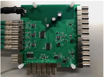
2.2 Detector Geometry

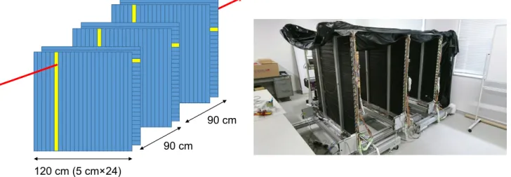
The detector part comprises the following three parts: plastic scintillators, photosensors, and support structures. Figure 2.2 depicts the geometry and a picture of the detector. The detector comprises three pairs of two layers. Each layer has 24 plastic scintillators (EJ-212, ELJEN TECHNOLOGY [19]) of 5 cm width, 2 cm thickness, and 120 cm length. The scintillators are

(24)

placed orthogonally to measure the hit position of a penetrating charged particle. Consequently, we can measure three positions of the incident particle using the detectors.

Notably, the photosensors, SiPMs (S13360-3050PE, Hamamatsu Photonics K. K. [20]), are attached to both the sides of each scintillator. The size, typical gain, and operating voltage are 3.0×3.0 mm², 1.7×10⁶, and 53 V, respectively. The gain of the SiPMs has the temperature dependence of 1.7%/^◦C. The SiPM is mounted on a board to be held on the scintillator, and it is optically coupled to the scintillator using a piece of silicone rubber (EJ-560, ELJEN TECHNOLOGY [21]).

Both the pair of the layers are supported by a 10-mm thick stainless plate between them.

Including the scintillators, their total radiation length is 2.0X₀. Therefore, the plates also play a role to reduce the backgrounds of the EM component.

120 cm (5 cm×24)

90 cm 90 cm

Figure 2.2: Detector overview. The left and right panels show the geometry and the picture of the detector, respectively.

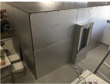
These detector components are covered by a housing that is made of aluminum frames and plywood walls. The housing can be decomposed into frames and walls. Therefore, we can transport and re-build them for outdoor usage. Figure 2.3 depicts the detector housing.

The width, length, and height of the housing are 2 m, 3 m, and 2 m, respectively. An epoxy glue (E2420, Konishi) was used to attach a heat-shielding insulation sheet (HM sheet, Einen [22]) to the wall. Consequently, the wall not only shielded from raindrops but also countered temperature variation.

2.3 Data acquisition system

The DAQ system comprises two parts. One is a product called the NIM EASIROC module [23]. We use one module per layer, i.e., six modules in total. The other part is a logic board developed for the muography system.

2.3.1 NIM EASIROC module

The NIM EASIROC module manages the SiPMs. It has two ASICs¹ called EASIROC to process signals from the SiPMs. A French high-energy physics group [24] developed this ASIC chip, which processes signals from 32 SiPMs. Accordingly, the module can manage 64 SiPMs.

1Application-specific integrated circuit.

(25)

Figure 2.3: Picture of the housing. The heat-shielding sheet covers the wall. The middle equipment is an air-conditioner to control the temperature for urgent needs.

In addition, the module can supply the operating voltages to them. The operating voltage can be adjusted to each SiPM within a range of 4.5 V.

An FPGA² controls the ASICs and manages the measured signals. We installed a firmware [25], which was developed for a neutrino experiment, on the FPGA. The firmware enables the module to measure four kinds of information of the 64 SiPM signals.

The module processes the signals from the SiPMs with three lines. Figure 2.4 depicts the overview of the circuit, and Fig. 2.5 explains the information measured by the module. The first line is processed using a high-gain amplifier and fast shaper. Two TDC-information types, i.e., leading and trailing edges of the waveform, are measured within a 1-ns interval. A slow shaper processes the remaining two lines using a high- or low-gain amplifier. The two lines precisely measure the pulse height with 12 bit. Using the two lines enables us to extend the dynamic range of the pulse height measurement. The FPGA collects the measured values and sends them to a PC via a computer network.

2.3.2 Logic board

To reject unnecessary events, the muography system records only those events wherein hits occur on all the layers. The system needs some logical processes to ensure coincidence in time among the hits. Although general-purpose modules can ensure this, they consume considerable power. In our case, a logical circuit using general-purpose modules consumed approximately 150 W. Therefore, we developed a special logic board depicted in Fig. 2.6.

The board takes a coincidence in the time of six layers by processing the signals from the NIM EASIROC modules. Subsequently, it outputs some signals to them to record data. Although the board is meant only for our use, it has suﬃcient performances: the latency of 20.5±0.9 ns and timing resolution of 0.3 ns. It consumes only 1.8 W because of the energy-saving chips with CMOS.

2.3.3 Monitor system

The temperature of the SiPMs is important, because their amplification factors are dependent on it. We developed a monitor system to record some environmental parameters. Figure 2.7

2Field-programmable gate array.

(26)

Figure 2.4: Overview of the NIM EASIROC module [23].

Pulse Height

High Gain

Low Gain t

threshold

T_trailing

t T_leading

TDC

Figure 2.5: Overview of the information recorded by the module.

(27)

Figure 2.6: Picture of the logic board.

depicts an overview. The monitor system has two kinds of sensors. One is an environmental sensor unit (BME-280, Bosch Sensortec), which measures the humidity, temperature, and atmospheric pressure in the housing. The other kind is a temperature sensor (LM61, Texas Instruments) to measure the temperature of the SiPMs. A sensor is attached to the jig of a SiPM, i.e., 48 sensors per layer and 288 sensors in total. An ADC chip (MCP3208, Microchip) converts eight analog signals from the sensors into digital values with a 14-bit resolution. By calibrating the digital values, we obtained the temperature resolutions of approximately 0.1^◦C.

A microcomputer (Raspberry Pi 3B, RS components) manages the six ADC chips and two environmental sensor units. The six microcomputers monitor the environmental parameters.

They send the data to the PC via a wireless computer network.

0.5 m Temp. Sensor

ADC Micro Computer

1.5 m

Temp./Humidity/Pressure Monitor

2 m

BME280 Board ADC Board

Temp. Sensor Micro Computer Board

PC Network

x8

x6 x2

x6

Figure 2.7: Overview of the monitor system and its pictures.

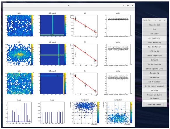
2.3.4 Control system

A PC manages the NIM EASIROC modules via a computer network. To control the modules, we developed a control system with a graphical user interface. The interface is primarily

(28)

based on Ruby. We also used C++ for analysis and data handling to boost computation.

Figure 2.8 depicts a picture of the display during an instance of data acquisition. During the data acquisition, the system provides an event display as a quick analysis. When a problem occurs, the system detects it and automatically restarts the data acquisition. Therefore, we need not frequently access the PC.

Figure 2.8: Display during a data-acquisition instance.

2.4 Power system

2.4.1 Power consumption

The detector, monitor, and control systems described above require electric power to function.

We measured their power consumption using a wattmeter, during a data-acquisition. Table 2.1 presents the power-consumption detail of the muography system. An energy-saving laptop PC consumes only 24 W. The total power consumed by the system is less than 100 W.

2.4.2 Power-generation and storage system

We constructed a power-generation and storage system. Six solar panels each with the power of 200 W (AT-MA200A, JAsolar) were used to generate the electricity. A charge controller (XTRA3415N-XDS2, EPEVER) was used to control them and charged 16 deep-cycle batteries (M31MF, AC Delco). The batteries could store the electric power of approximately 22 kWh.

A DC–AC inverter (CPT-3000-148, COSUPER) were used to supply electricity to the other systems. However, we should assume the case wherein the batteries become empty due to bad weather. In such a case, a dynamo (HPG3000i, Wakita) provides the electricity, and it enables us to charge the batteries in bad weather.

(29)

Item The number Power consumption [W]

PC 1 24

Logic board 1 1.8

EASIROC Modules 6

Network Hub 2 53.9

Monitor System (six microcomputers) 1 10.8

Router 1 8

Total 98.5

Table 2.1: Detail of the power consumption of the muography system.

As a demonstration, we tested the power system using only three solar panels from June 4th to 5th, 2019. Figure 2.9 depicts the corresponding result. The system generated the total power of 2.1 and 2.9 kWh on June 4th and 5th, 2019, respectively. However, using six solar panels, we can expect the total power of 4.2 and 5.8 kWh, respectively. The power diﬀerence between both the days is attributed to the weather, which was sunny, partly cloudy, and rainy on the 4th and was sunny on the 5th of June, 2019. Consequently, the power system satisfies the power-consumption demand of the muography system, i.e., 2.4 kWh/day.

0.0 1.0 2.0 3.0 4.0 5.0 6.0

06/03 12:00 06/04 00:00 06/04 12:00 06/05 00:00 06/05 12:00 06/06 00:00

Total Gerated Power [kWh]

Date

Figure 2.9: Result of the power-generation test.

(30)

Chapter 3 Reconstruction method and its performance

The measured values were used to reconstruct the incident particles. In the reconstruction, the dependence of the detectors was taken into account, and the real values were obtained. In this chapter, we show some methods and reconstruction performance.

3.1 ADC distribution

A combination of the high-gain (HG) and low-gain (LG) ADC values enables us to extend its dynamic range. The left part of Fig. 3.1 depicts a correlation between the two aforementioned values. They are fitted using a linear function as follows:

x_HG =p₀+p₁·x_LG, (3.1)

where x_HG, x_LG, and p_i (i = 0,1) denote the HG value, LG value, and fitting parameters, respectively. Here, we define a combined ADC value using both the values. Because the HG value saturates at approximately 3000 ch, we use it as the combined ADC when it is less than the threshold of 2500 ch. Otherwise, the LG value is converted to the combined ADC to be equivalent to the HG value. Therefore, the combined ADC is given as

x_comb.= {

x_HG (x_HG <2500),

p₀+p₁·x_LG (x_HG ≥2500). (3.2)

where xcomb. denotes the combined ADC value.

Figure 3.2 depicts a distribution of the combined ADC value. In the figure, two peaks are observed. The left peak at approximately 800 ch, corresponds to the pedestal. It spreads due to the noise on the channel, and its mean value depends on the channel. The other peak, which is the broader one, is the MIP peak. It obeys the Landau distribution convoluted with the resolution of the channel. Hereinafter, we refer to the pedestal subtracted ADC as the ADC value.

3.1.1 Photon yield

We must confirm whether the scintillators have suﬃcient photon yields. To evaluate the yield, we calibrated the ADC. Because SiPMs can count the number of photons, we can estimate the photon yield of each SiPM by using the ADC values. Figure 3.3 depicts an ADC distribution.

(31)

LG-ADC LG-ADC

HG-ADC Combined ADC

(a) (b)

Figure 3.1: (a) Correlations between HG ADC and LG ADC (left) and (b) between LG ADC and combined ADC (right). HG ADC less than 2500 ch is plotted here because it saturates at approximately 3000 ch.

adc_combined Entries 1443922

Mean 896.7

Std Dev 391

0 2000 4000 6000 8000 10000 12000 14000 16000

1 10 10

2

10

3

10

4

10

5

10

6

adc_combined Entries 1443922

Mean 896.7

Std Dev 391

hadc[0][12]

ADC

Entries

MIP peak

Saturation of HG

Saturation of LG Pedestal peak

Figure 3.2: Histogram of the combined ADC. The red histogram shows the HG component, and the blue one the combined ADC value.

(32)

There exist many peaks with a narrow interval, which correspond to single photons. We estimated the number of photons at the MIP peak,N_{pe,M IP}, using the following equation:

N_{pe,M IP} =ADC_{M IP}/∆ADC_pe, (3.3)

whereADCM IP denotes the value at the MIP peak, and ∆ADCpe is the interval of the narrow peaks. The histogram of the photon yields is depicted in Fig. 3.4. Consequently, the SiPM detects 29±6 photons/MIP. This value is suﬃciently high to distinguish a hit on the scintillator from noise events.

0 500 1000 1500 2000

10 10

2

10

3

10

4

10

5

h_2_15

h_2_15 Entries 934011 Mean 75.11 RMS 315.4

h_2_15

ADC Value

En tr ie s

Figure 3.3: Pedestal subtracted ADC distribution. The peaks with the narrow interval shown with the triangles correspond to the photons. The right broad peak originates from MIP events.

3.1.2 Reconstruction of energy deposits on the scintillators

Because an ADC value represents the energy loss of a particle on a scintillator, each scintillation counter must be calibrated to convert the ADC value to the energy loss. The ADC value includes two dependences shown in the following. In this section, we describe the correction of the dependence and reconstruction of the energy deposit.

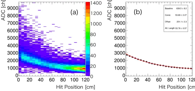
Hit-position dependence

Scintillators wrapped with reflector film propagate produced photons. They lose the photons despite their high transparency and the high-reflectivity of the reflectors. To measure the energy deposit, we must correct this attenuation eﬀect. Figure 3.5 (a) depicts the scattered plot of the ADC values and hit position. It is evident that the value has hit-position dependence.

We corrected the dependence using an exponential function of the hit position, x_hit, which is written as

A_pos.(x_hit) =ADC_oﬀset+ exp (

−x_hit−x_oﬀset L_att.

)

, (3.4)

(33)

h

Entries 282 Mean 28.72 RMS 5.737

# of Photons

15 20 25 30 35 40 45

Entries

0 5 10 15 20 25 30

h

Entries 282 Mean 28.72 RMS 5.737

Figure 3.4: Histogram of the photon yields.

where ADC_{of f set}, L_att., and x_{of f set} denote an oﬀset of the ADC value, attenuation length, and oﬀset of the hit position, respectively. Figure 3.5 (b) depicts the result of the fitting. We can see that the function satisfactorily reproduces the dependence. Similarly, the hit position dependence in all the scintillators was corrected individually.

Temperature dependence

The gain of an SiPM decreases in proportion to its temperature. The temperature measured by the monitor system is used to correct the dependence. Figure 3.6 depicts a correlation between the measured temperature and the ADC values at the MIP peak of an SiPM. We corrected the temperature dependence by using the following linear function:

Atemp.(T) =p0+p1T, (3.5)

whereT denotes the measured temperature, and p_i (i= 0,1) the free parameters. The red line shows the function, which satisfactorily reproduces the dependence. All the SiPM signals were individually corrected in the same manner.

Reconstruction of energy deposit on a scintillator The ADC values are corrected using the following formula:

ADC_cor. = ADC

A_pos.(x_hit)·A_temp.(T). (3.6)

The corrected ADC values are converted to the energy deposit in MeV. To perform the conversion, we consider not only the conversion factor but also detector resolutions. In the following, we show the procedure to determine the aforementioned two parameters, i.e., conversion factor and detector resolutions.

(34)

ADC [ch]

Hit Position [cm]

ADC [ch]

Hit Position [cm]

1400 1200 1000 80 60 40 20 0

(a) (b)

Figure 3.5: (a) Example of the hit-position dependence. The horizontal axis represents the hit position on the scintillator and the vertical axis the pedestal subtracted ADC value. (b) The right part shows the slices along the Y-axis and the fitting result.

ADC/Apos.(xhit) [a.u.]

Temperature [℃]

Figure 3.6: Temperature dependence of an SiPM. The horizontal axis represents the temperature measured using the temperature sensor, and the vertical axis represents the ADC value at the MIP peak after the hit-position correction.

(35)

First, we measure the ADC values of each SiPM with cosmic ray muons and prepare for a histogram of the corrected ones. Next, we prepare for another histogram of the energy deposit on the scintillator using a Monte Carlo (MC) simulation, which will be detailed in the next chapter. Then, we determine the conversion factors and the detector resolutions to match the corrected ADC values and the estimated energy deposit. Figure 3.7 depicts the histograms of the corrected values and the energy deposit estimated using the MC. The blue line in the right figure represents the fitting result. Although there exists a small discrepancy between them around the corrected ADC of 4 a.u., the line agrees with the data. Consequently, their detector resolution is 0.63±0.04 MeV, as depicted in Fig. 3.8 This resolution is consistent with the statistic estimation of the number of photons detected.

mc_0_6

Entries 51014 Mean 4.474 Std Dev 1.414

0 5 10 15 20 25 30 35 40 45 50

-10

10

-9

10

-8

10

-7

10

-6

10

-5

10

-4

10

-3

10 ^mc_0_6

Entries 51014 Mean 4.474 Std Dev 1.414

mc_0_6

0 2 4 6 8 10 12 14

edep_data_var 10

102

103

Projection of conv_gaus

Data_0_6

Energy Deposit [MeV] ADCcor[a.u.]

Figure 3.7: Histograms of the ADC and the energy deposit on the scintillator. The left shows the energy deposit. The right shows the ADC measured with cosmic ray muons, and the blue line represents the fitting result.

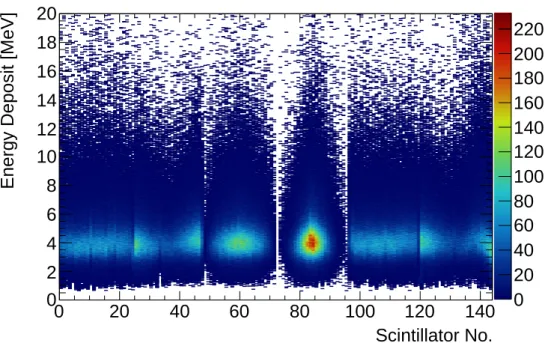
Reconstruction of energy deposit on a layer

The hit scintillators provide the total energy deposit on a layer. To discriminate a hit on a scintillator from noise, we use an energy threshold of 0.4 MeV. Figure 3.9 depicts the reconstructed energy deposit. Here, we applied a condition that a particle hits one or adjoining two scintillators on all layers, to remove multi-hit events. We can see the MIP peaks at approximately 4 MeV, which is 10 times higher than the threshold. Therefore, the threshold is suﬃciently low to discriminate hit events.

3.2 Time information

3.2.1 Reconstruction of the hit timing

The module records the time when an SiPM detects scintillation photons. However, the measured time on the SiPM, tSiPM,measure, involves ∆t_delay, sum of delay eﬀects. In our case, the measured time is written as

tSiPM,measure = t_SiPM,hit+ ∆t_delay (3.7)

= (t_sc.,hit+ ∆t_prop.) + (∆t_time-walk+ ∆t_oﬀset), (3.8)

(36)

0.3 0.4 0.5 0.6 0.7 0.8 0.9 Energy Resolution [MeV]

0 5 10 15 20 Entries 25

Energy Resolution

Energy Resolution Entries 144 Mean 0.6259 Std Dev 0.03637

Energy Resolution

Figure 3.8: Histogram of the energy resolutions.

0 20 40 60 80 100 120 140

Scintillator No.

0 2 4 6 8 10 12 14 16 18 20

Energy Deposit [MeV]

0 20 40 60 80 100 120 140 160 180 200 220

edep[]:hit_seed_ch[Iteration$]+Iteration$*24 {Track_NumOfCandidates==1}

Figure 3.9: Distribution of the reconstructed energy deposit. The horizontal axis represents the scintillator channels.

(37)

wheretsc.,hitdenotes the hit time on the scintillator, ∆tprop.the delay due to photon propagation,

∆t_time-walk is the delay due to pulse-height dependence (called time walk), and ∆t_offset the offset of the measured time. The following subsections describe the methods to correct the aforementioned delay effects and reconstruct the hit timing on a scintillator.

Hit-position dependence

The photon propagation in scintillators results in a delay in the detection time on an SiPM.

First, we correct the delay. The left part of Fig. 3.10 depicts a correlation between the hit position on a scintillator and the hit timing delay of an SiPM. The correlation is fitted using the following linear function:

∆t_prop.=p₀+p₁·x_hit, (3.9)

where xhit denotes the hit position, and pi (i= 0,1) the fitting parameters. As depicted in the figure, the function describes the relation well. After correcting the dependence, we correct the other dependences.

Hit Position [cm]

TDC [ns]

Hit Position [cm]

TDC [ns]

200 400 600 800 1000

0

Figure 3.10: Hit-position dependence of the TDC. The vertical axis represents the diﬀerence between the measured time on the SiPM and the one estimated using the other layers. The horizontal axis represents the hit position.

Pulse-height dependence

When a signal crosses a threshold, the crossing time depends on the pulse height of the signal, as depicted in Fig. 3.11. This dependence is called time walk. However, the NIM EASIROC module cannot record the pulse height generated using the fast shapers. Instead of the pulse height, we use another value, which is time-over-threshold (TOT), to correct the time walk.

The TOT is the time diﬀerence between the leading edge and the trailing edges, and has strong correlation to the pulse height. Figure 3.12 depicts the correlation between the TOT and the delay of the time walk. Here, we defined the delay, ∆t_time-walk, as the time diﬀerence between the time of the leading edge and the hit time on a scintillator estimated by other layers. We corrected the delay by assuming the following function:

∆t_time-walk =p₀+ p₁

TOT−p₂, (3.10)

with three fitting parameters, p_i (i = 0,1,2). The red line on the left figure represents the fitting result, which reproduces the time walk. The right figure depicts the distribution of the diﬀerence between the time after the time walk correction and the estimated hit time

(38)

on the scintillator. Because of the time walk correction, the distribution obeys the Gaussian distribution with the mean value of zero.

threshold

T₁

time

T_det T₂

waveform1

waveform2

Figure 3.11: Outline of the time walk correction. T_det denotes the time when an SiPM detects photons, and T₁ (T₂) denotes the time when a signal of waveform1 (wavefomr2) crosses the threshold. The crossing time depends on the pulse height.

TOT [ns]

ΔT [ns]

Figure 3.12: Result of the time walk correction. The left shows the correlation between the TOT and ∆t_time-walk. The right shows the distribution of ∆t_time-walk after the hit-position and the time walk correction.

Channel dependence

Each TDC channel has an intrinsic offset due to cable delay and other sources. As the last correction, we tuned the offset, ∆t_offset, by using cosmic ray particles. Because their velocity was almost equal to that of light, the offset was determined to match the measured hit timing to the estimated one by the other TDC values.

Kyushu University Institutional Repository

九州大学学術情報リポジトリ