PROTON ACCELERATION AND ITS ENERGY SPECTRA DURING THE COALESCENCE OF TWO CROSS CURRENT
LOOPS
Laboratory for Plasma Astrophysics, Faculty of Engineering Kazuaki Shimada and Jun-ichi Sakai [email protected]
We investigate the plasma dynamics during coalescence of two cross current loops by using a resistive three-dimensional MHD simulation code, particularly paying attention to find the most effective electromagnetic fields for the production of high-energy protons. Next we investigate the orbit of many protons in the electromagnetic fields obtained from the MHD simulations. We found that the proton acceleration is more efficient than the case of two parallel loops coalescence. It is shown that the maximum proton energy is about 25 MeV and exceeds the energy (2.223 MeV) of the observed prompt nuclear de-excitation lines of gamma-ray and the proton energy spectrum is a power-law type with an indexof about 2 - 2.3. The simulation results imply that proton-associated gamma-ray sources are located near the footpoints with magnetic north polarity. We found that strong proton acceleration leading to the observed prompt line gamma-ray emissions can be realized only when there occurs the complete magnetic reconnection where both poloidal and axial magnetic fields reconnect.
Key words : Sun: flares-Sun: loop coalescence flare- Sun: proton acceleration
1 Introduction
When energetic protons accelerated during impul- sive flares collide with solar atmosphere, they pro- duce excited nuclei, which emit prompt nuclear de- excitation lines, as well as secondary neutrons and positrons that results in the delayed 2.223 MeV neutron-capture and 511 KeV positron-annihilation line emission. In most strong flare events the time profile of the prompt gamma-ray line emis- sion is observed to be very similar to that of the bremsstrahlung hard X-rays emitted by energetic electrons. This suggests that the acceleration and propagation of the flare-accelerated protons and electrons are closely related. The most typical event among them is the 1980 June 7 flare observed by the SMM (Forrest and Chupp 1983), which flare was explained by the current loop coalescence model (Tajima et al. 1982; Sakai & Ohsawa 1987; Sakai
& De Jager; 1996; Aschwanden 2002). Sakai & de Jager (1996) gave a review of the high-resolution observations of solar plasma loops with simulations of current-carrying loops and tried to arrive at the understanding of solar flare phenomena.
As proposed by de Jager (1988) and Sakai & de Jager (1991), there are three phases of acceleration
in a fully developed eruptive/dynamic flare. The relevant observations regarding the first two phases are:
(1) the acceleration times of electrons and protons to energies of the order of one MeV are of the order of a second.
(2) MeV protons are accelerated nearly simultane- ously with MeV electrons.
Many theoretical works (Forman et al. 1986; Sim- nett 1995; Sakai & de Jager 1996; Miller et al.1997;
Aschwanden 2002) to explain the above observa- tional requirements have been done.
However, the location, size and geometry of the accelerated proton collision region remains un- known until now. Recent paper by Hurford et al.
(2003) presents the first gamma-ray images of a so- lar flare taken from the Reuven Ramaty High En- ergy Solar Spectroscopic Imager (RHESSI) for the X4.8 flare of 2002 July 23. The result shows that the centroid of the 2.223 MeV image was found to be displaced by 20 ± 6 arcsec from that of the 0.3-0.5 MeV, implying a difference in acceleration and /or propagation between the accelerated elec- tron and proton population near the Sun. The fact that proton-associated gamma-ray source does not
coincide with the electron-bremsstrahlung sources suggests that the protons would be accelerated in one direction by the DC electric field and could subsequently interact in spatially separated sources.
Therefore it is now important to investigate in de- tails the proton acceleration processes for different types of flares.
Sakai (1990a, 1990b) showed that, during 3D X- type current loop coalescence and under suitable as- sumptions of the size and other physical parameters in the region of acceleration, protons and electrons may be accelerated promptly (i.e., within less than 1 s) to≈100 GeV and≈100MeV, respectively. De Jager & Sakai (1991) showed that the duration of impulsive phase bursts (5-25 s) observed during the impulsive phases of flares can be explained quanti- tatively by the mechanism of X-type current-loop coalescence. Sakai (1992) developed a model for long-duration gamma-ray/proton flares (the ’grad- ual GR/P flares’) in order to explain prompt pro- ton and electron acceleration during the impulsive phase. He determined the electric fields during the implosion phase of the current sheet from the MHD equations, and investigated the motion of test pro- tons and electrons. Results showed that, under rea- sonable assumptions of the size and velocities in the reconnection area, both protons and electrons can be accelerated promptly within 1 s to ∼ 70 MeV and∼200 MeV, respectively. However, the above previous works did not give the energy spectrum of accelerated particles.
Mori et al. (1998) investigated the behavior of protons near an X-type magnetic reconnection re- gion by numerical simulations. The magnetic field is taken to be hyperbolic and time stationary with a uniform electric field perpendicular to the magnetic field. They also studied the effects of the magnetic field along the uniform electric field. They found from many parametric runs that the energy spec- trum of accelerated protons near an X-type mag- netic reconnection region is universal with a power- law spectrum E−γ, where the power-law index γ is about 2.0-2.2. The acceleration time of protons with the energy range of 1-20 MeV is very rapid and within∼ 102ω−1ci which is much less than 1 s for solar flare plasmas. Heerikhuisen et al. (2002) and Craig et al. (2002) investigated the proton dy- namics under a self-consistent MHD reconnection solution and found that the proton energy spectra approximates a power law E−1.5 nonrelativisti- cally, but steepens slightly at the higher energies.
Hamilton et al. (2003) studied the proton energy spectra under the model fields obtained from so-
lutions of the linearized MHD equations for recon- necting region. They showed that in some cases the energy distributions exhibit a bump-on-tail in the MeV range, but in general, the shape of the distribution is sensitive to the model parameters.
The previous model fields used during coalescence process to obtain the proton energy spectrum were limited by the spatial simple configurations near the reconnection region and by no self-consistent MHD solutions.
Sakai and Shimada (2004) investigated the plasma dynamics during coalescence of two parallel current loops by using a resistive three-dimensional MHD simulation code and the orbits of test pro- tons under the most effective electromagnetic fields obtained from the MHD simulations. They found that for the proton acceleration the co-helicity re- connection is more efficient than the case of counter- helicity reconnection. The protons can be acceler- ated mostly in one direction along the loop axis near where magnetic reconnection occurs. They also showed that the proton energy spectrum is nei- ther pure power-law type nor pure exponential type.
They proposed one of possible scenario to explain the above recent observation as follows. The single loop is supposed to be disrupted by the mechanism recently proposed by Sakai et al. (2002), then the disrupted part of the loop with high energy protons as well as hot thermalized protons could move up and then interact with overlying other loop. The in- teraction between the ascending magnetized plasma blobs and other loop can lead to magnetic recon- nection in the interaction region, where the proton could be accelerated more by the inductive elec- tric field associated with the magnetic reconnection mostly in one direction along the guiding magnetic field.
In the present paper we investigate the plasma dynamics during coalescence of two cross current loops by using a resistive three-dimensional MHD simulation code developed by Sokolov et al. (1999, 2002), particularly paying attention to find the most effective electromagnetic fields for the production of high-energy protons. Next we investigate the or- bit of many protons in the electromagnetic fields obtained from the MHD simulations. We found that the proton acceleration is more efficient than the case of two parallel loops coalescence investi- gated by Sakai and Shimada (2004). It is shown that the maximum proton energy is about 25 MeV and exceeds the energy (2.223 MeV) of the ob- served prompt nuclear de-excitation lines of gamma- ray and the proton energy spectrum is a power-law
type with an index of about 2 - 2.3. The simula- tion results imply that proton-associated gamma- ray sources are located near the footpoints with magnetic north polarity.
In§2 we present our methods to obtain the pro- ton energy spectra during coalescence of two cross current loops. In§3 we present our MHD simulation results to obtain the most effective electric fields for accelerating the protons. In§4 we investigate many proton orbits under the electromagnetic fields dur- ing the coalescence to find their energy spectra. In final section we summarize our results.
2 Methods of simulations
In this section we describe two methods of simula- tion to obtain the energy spectrum of the protons accelerated during the coalescence of two cross cur- rent loops. Fig.1 shows a schematic picture (lower figure) of two current loops (loop1 and loop2) that are crossing with an angle of 90 degree and the coor- dinate system (upper figure) used in the simulation.
x y
z
Bz
By
B B loop1
loop2
N S
N
S
loop2 loop1
j
j
Figure 1: A schematic picture (lower figure) of two current loops (loop1 and loop2) that are crossing with an angle of 90 degree and the coordinate sys- tem (upper figure). The system size is Lx = 300, Ly=Lz= 200.
Firstly we present briefly a model of two cross loops coalescence flare by using a three-dimensional resistive MHD simulation to obtain the electromag-
netic fields during the loop coalescence. Next we present the simulation method to obtain the orbits of many protons under the electromagnetic fields obtained from the MHD simulations.
2.1 Resistive MHD simulation
A resistive 3-D MHD code with recently proposed Artificial Wind(AW) numerical scheme (Sokolov et al. 1999, 2002) with splitting over the spatial coor- dinates is employed. The basis of the AW scheme is the fact that fundamental physical invariance, Galilean (or more general, Lorentz) invariance, al- lows to solve the governing equation in different steadily moving frame. The principle of the AW scheme is that the frame of reference may be cho- sen in such a way that the flow under simulation is supersonic there. The problem of upwinding be- comes trivial and considerably facilitated versions of discontinuity-capturing schemes may be employed.
An extra velocity (Artificial Wind) is added to the velocity of the flow under simulation when the sys- tem of coordinates is changed.
The MHD equations are numerically solved in a conservative form as follows:
∂ρ
∂t + ∂
∂xi
(ρVi) = 0, (1)
∂(ρVi)
∂t + ∂
∂xj
ρViVj+ (p+B2)δij−2BiBj
= 0,
(2)
∂Bi
∂t + ∂
∂xj
(VjBi−ViBj) = 1 Rm
∂2Bi
∂x2j , (3)
∂
∂t(ρV2
2 + p
γ−1 +B2)+
∂
∂xi
Vi(ρV2
2 + γp
γ−1+ 2B2)−2BiBjVj+qi
= 0, (4) where, ρ, Vi, p and Bi are the density, velocity, pressure, and magnetic field,γis the adiabatic con- stant, which is taken to beγ= 5/3,Rmis the mag- netic Reynolds number, δij is a unity tensor and qi is a dissipative energy flux . The density, pres- sure, velocity and magnetic field are normalized by ρ0, p0,
p0/ρ0and B0=√
8πp0, respectively.
For resistive MHD with a large but finite value of Rm the energy equation Eq.(4) should be ob- tained as a sum of the equation for plasma energy, in which the Joule heating term is present as fol- lows: (c∇×B)(4π)2σ2 and the equation for magnetic energy
which is given by the Eq.(4) multiplied by the mag- netic fieldBi/(4π), all the variables are not normal- ized here andσ is a conductivity. The dissipation of the magnetic field energy is hence given by the term as follows: (4π)c22σBi∆Bi. So in the Eq.(4) for the total energy the Joule heating is compensated by the magnetic energy dissipation in a following way:
c2 (4π)2σ
Bi∆Bi+ (∇ ×B)2
= c2
(4π)2σ∇·[B×∇×B]. (5) So the resistive dissipation in the equation of en- ergy in present only in a form of the additional dis- sipative energy flux, which, in normalized variables, may be written as follows: qi(m)=R−1m ∂x∂j(2BiBj− B2δij). The dissipative energy flux due to heat transfer may be also taken into account in a usual form:q(h)i =λij ∂
∂xj
p
ρ. For the sake of simplicity here we fully neglect the non-diagonal part of dissipa- tive energy transfer tensor and substitute all the tensors in qi for unity tensors: BiBj = B2δij/3, λij = λllδij/3. The numerical simulation shows that the influence of the dissipative energy flux is insignificant, so we do not try to take it more care- fully into account. Finally we admit the dissipative hydrodynamic flux to be as follows:
qi= ∂
∂xi
− B2 3Rm−λp
ρ
. (6)
The magnetic Reynolds numberRm= 1.3×10³and the heat transfer constantλ= 2.5×10⁻⁴ are used in simulation. Radiating boundary conditions were used for all directions.
Here we take a system size as Nx = 300 and Ny=Nz= 200, as shown in Fig.1. The two current loops where the loop1 is located parallel along the z-axis, while the loop2 is located parallel along the y-axis. Both loops are assumed to be in an equilib- rium state, in which the magnetic field and pressure for each loop are given as
Bx=q2B02(z−zc2)
a e−(ra2)2+q1B01(y−yc1)
a e−(ra1)2, (7) By=B02e−(ra2)2−q1B01(x−xc1)
a e−(ra1)2, (8) Bz=B01e−(ra1)2−q2B02(x−xc2)
a e−(ra2)2, (9) pi=
q2i 2 −q2ir2i
a2 −1
e−2(ria)2+ 0.55, (10)
where r1 =
(x−xc1)2+ (y−yc1)2, r2 = (x−xc2)2+ (z−zc2)2, and the centers of the two flux tubes with a radius a = 30 are (xc1, yc1) = (105,100) and (xc2, zc2) = (195,100). The density profile is the same as the pressure. The twist param- eterqi isq1=q2= 1 andB01=−1 andB02= 1.0.
The plasma betaβ in the center of the two loops is 0.06.
2.2 Simulation of proton dynamics
By using the electromagnetic fields obtained from the above MHD equations during coalescence of two parallel current loops, we investigate the protons dynamics to obtain their energy spectrum. The normalized relativistic equations of the motion of a proton is given by
du
dt =E+u×B
γ , (11)
dx dt = Rv
γ , (12)
where the proton velocity v = γ−1u, the electric field E, and the magnetic field B are normalized by Alfv´en velocity VA , E0 = VAB0/c, and B0, respectively. The time is normalized by the pro- ton cyclotron frequencyωci, and the length is nor- malized by the distance over which the fields are changed across the loop radius (a), respectively.
The Lorentz factorγis given byγ= (1 +A2u2)1/2, whereA=VA/c. The parameterRin Eq.(3) is de- fined byR=VA/(ωcia). In our simulation we take A= 1/300 andR= 10−8.
To advance particle under the guidance of elec- tric and magnetic fields through solving the motion equation numerically, we used a centered-difference form of the Newton-Lorentz equations of motions (Buneman 1993; Birdsall&Langdon 1991), namely
unew−uold = qδt m [E+ 1
2Γ(unew+uold)×B], (13)
where q is the charge of a particle, m is the mass of a particle, and δt is the calculate time step, re- spectively. As it stands, the equation for unew is implicit. We choose the method proposed by Boris (1970) to obtain a simpler explicit solution using several steps.
The protons are randomly distributed with one proton per cell. The initial velocity distribution function for protons is Maxwellian with the thermal velocity vth = 0.4VA. The simulation time step is ωciδt= 0.05. The boundary conditions for protons are open in the x-, y- and z-directions.
3 Simulation results of two cross loops coalescence
The basic physical evolution of reconnection be- tween two cross loops was investigated by several authors (see, Sakai 1990b; Sakai & de Jager 1997
; Linton et al. 2001). Each of the two cross cur- rent loops is in an equilibrium state as long as the distance between them is much greater than loop radiusa. While the loops approach to each other, they are no longer in the equilibrium state and the whole non-equilibrium system tends to a new equi- librium state. In more details, due to attraction, the two initially static current loops begin to move and approach to each other. Then they meet, merge, with sling-shot magnetic reconnection. We men- tion here that only when there occurs the complete magnetic reconnection where both poloidal and ax- ial magnetic fields reconnect, high energy protons are generated.
Here we present the simulation results of dynam- ics of two cross current loops, especially paying at- tention to where and which stage the most strong electric fields are formed to accelerate protons. Fig.
2 shows the time evolution of the isosurface of to- tal magnetic field intensity with|B|= 0.26 during the collision of two cross current loops: (a) t = 0, (b)t = 35τA, (c) t = 59τA, and (d) t = 82τA. As shown later, the most strong electric field appears at t= 59τA shown in Fig.2(c) where magnetic recon- nection occurs. Therefore we investigate the spa- cial structures of the electric and magnetic fields at t= 59τA shown in Fig.2(c).
Figs.3 shows the spacial structures of the electro- magnetic fields att= 59τAin Fig.2(c) that are used in the calculation of test proton orbits. Fig.3(a) showsBx(gray scale) and vector plot of By-Bz on x= 150. Fig.3(b) showsBy(gray scale) and vector plot ofBx-Bz ony= 100. Fig.3(c) shows Ex(gray scale) and vector plot ofEy-Ezonx= 150. Fig.3(d) showsEy(gray scale) and vector plot ofEx-Ez on y= 100.
The most important electric field leading to the proton acceleration is the parallel component to the local magnetic field that is generated near the region where magnetic reconnection occurs due to finite resistivity. To find such a region, we calculate the spacial value of the scalar productE·B. Fig.4(a) shows the spacial value of the scalar productE·B in thex−zplane ony= 100 att= 59τA. Fig.4(b) shows the spacial value of the scalar productE·Bin they−zplane onx= 150 att= 59τA. The black
x y
z
x
y z
x
y
z
x y
z
(a) (b)
(c) (d)
Figure 2: The time evolution of the isosurface of total magnetic field intensity with |B|= 0.26 dur- ing the collision of two current loops: (a)t= 0, (b) t= 35τA, (c)t= 59τA, and (d) t= 82τA.
-0.2 -0.1 0.0 0.1 0.2
0 100 200
0 100 y200
z
Bx
-0.1 0.0 0.1 0.2 0.3 0.4
0 100 200 300
0 100 200
x z
= 0.5
By
= 0.28
0 100 200 300
0 x
-0.15 -0.10 -0.05 0 0.05 Ey
0 100 y200
0 100 200z
-0.36 -0.24 -0.12 0 0.12 0.24 0.36 Ex
= 0.2
(a) (b)
(c) (d)
Figure 3: The spacial structures of the electromag- netic fields at t= 59τA in Fig.2(c) that are used in the calculation of test proton orbits. (a) Bx(gray scale) and vector plot of By-Bz on x = 150. (b) By(gray scale) and vector plot ofBx-Bzony= 100.
(c) Ex(gray scale) and vector plot of Ey-Ez on x= 150. (d)Ey(gray scale) and vector plot ofEx- Ez ony= 100.
region shows that the induced electric field is almost parallel to the local magnetic field, while the white region shows the region where the electric field is perpendicular to the local magnetic field. Therefore we conclude from the MHD simulation that near the magnetic reconnection region there appears strong longitudinal electric field along the local magnetic field that may play an important role for the proton acceleration.
0 100 200 300
0 100 200
x z
-0.002 -0.0015 -0.001 -0.0005 0
0 100 y 200
0 100 200z
0 -0.0005 -0.001 -0.0015
(a)
(b)
Figure 4: (a) The spacial value of the scalar product E·B in the x−z plane ony = 100 at t = 59τA. (b) The spacial value of the scalar productE·Bin they−zplane onx= 150 att= 59τA. The black region shows that the induced electric field is almost parallel to the local magnetic field, while the white region shows the region where the electric field is perpendicular to the local magnetic field.
4 Proton acceleration and its energy spectrum
In this section we present simulation results of dy- namics of many test protons under the MHD elec- tromagnetic fields att= 59τA discussed in the pre- vious section. First of all we present the proton energy spectra in Fig.5, where the energyE is nor- malized asE = (Vx2+Vy2+Vz2)/VA2.
Fig.5(a) shows the proton energy spectra at ωcit= 500 where the power law index is about 3.6 in the high energy region. Fig.5 (b) shows the pro-
ton energy spectra atωcit= 1500, where the power law index is about 2.3 in the high energy region.
Fig.5(c) shows the energy spectra at ωcit = 2500, where the power law index is about 2.0 in the high energy region. If we take the Alfv´en velocity as about 1000km, then the energy E = 102,103 cor- respond to 1M eV and 10M eV, respectively. The maximum proton energy reaches about 25M eV at ωcit= 2500.
0 1 2 3 4 5 6
0 1 2 3 4
log10f
log10E (1) (2) (3)
Figure 5: Proton energy spectra: (a) atωcit= 500 where the power law index is about 3.6 in the high energy region, (b) at ωcit= 1500, where the power law index is about 2.3 in the high energy region, (c) atωcit= 2500, where the power law index is about 2.0 in the high energy region.
To see the direction of the proton acceleration, we show the proton velocity distribution functions at ωcit = 2500 in Fig.6, where Figs.6(a)-(c) show the x-direction, y-direction, and z-direction, respec- tively. As seen in Fig.6(b), the protons in the loop 2 can be accelerated to the negative y-direction, while the protons in the loop 1 can be accelerated to the positive z-direction, as seen in Fig.6(c). The reason why the protons in the loops can be accelerated in one direction is investigated in the following analy- sis.
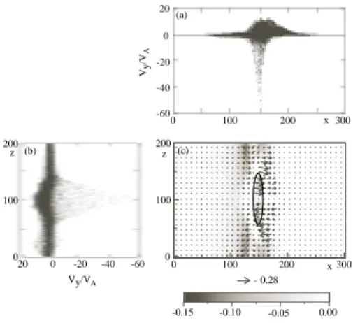
In Fig.7 we show the phase space plots of pro- tons at ωcit = 2500, where Fig.7(a) shows the plot of x-Vy and Fig.7(b) shows the plot of z-Vy. Fig.7(c) show the spacial structure of the electric field, Ey(gray scale) and the vector plot of Ex-Ez
ony= 100, where the elliptic region corresponding to Fig.4(a) shows the region of the loop 2 that the proton acceleration is dominant in the negative y- direction. In Fig.8 we show the phase space plots of protons atωcit= 2500, where Fig.8(a) shows the plot of y-Vy and Fig.8(b) shows the plot of z-Vy. Fig.8(c) show the spacial structure of the electric field, Ex(gray scale) and the vector plot of Ey-Ez
onx= 150, where the elliptic region corresponding
0 20 40 60 80 -20
-60 -40 -800 1 2 3 4 5 6 7 0 1 2 3 4 5 6 7 0 1 2 3 4 5 6
7 (a)
(b)
(c) Vy/VA Vx/VA
Vz/VA log10flog10flog10f
Figure 6: Proton velocity distribution functions of (a) the x-direction, (b) y-direction, and (c) z- direction atωcit= 2500. The protons in the loop 2 can be accelerated to the negative y-direction, while the protons in the loop 1 can be accelerated to the positive z-direction.
to Fig.4(b) shows the region that the proton accel- eration is dominant in the negative y-direction. As seen in the elliptic region the electric field vectors are dominantly to the negative y-direction. From the above analysis we conclude that the protons in the loop 2 are accelerated mostly to the negative y-direction.
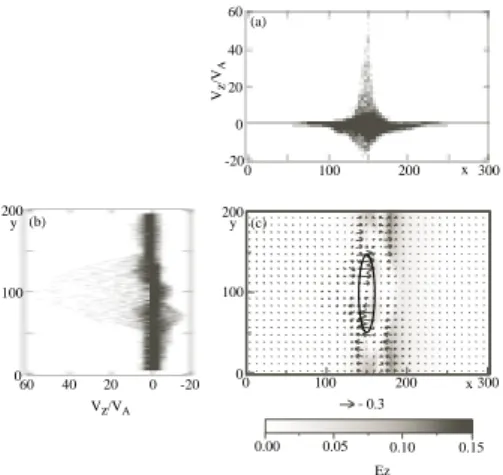
Next we examine the protons in the loop 1. Fig.9 shows the phase space plots of protons at ωcit = 2500, where Fig.9(a) show the plot of x-Vz and Fig.9(b) show the plot ofy-Vy. Fig.9(c) shows the spacial structure of the electric field,Ez(gray scale) and the vector plot ofEx-Ey onz= 100, where the elliptic region corresponding to Fig.4(a) shows the region of the loop 1 that the proton acceleration is dominant to the positive z-direction. fig.10 shows the phase space plots of protons at ωcit = 2500, where Fig.10(a) shows the plot ofy-Vzand Fig.10(b) shows the plot ofz-Vz. Fig.10(c) shows the spacial structure of the electric field, Ex(gray scale) and the vector plot of Ey-Ez on x = 150, where the elliptic region corresponding to Fig.4(b) shows the region where the proton acceleration is dominant to the positive z-direction along the loop 1. From the above analysis we conclude that the protons in
0 100 200
20 0 -20 -40 -60
Vy/VA z
0 100 200 300
20 0 -20 -40
-60 x
Vy/VA
Ey (a)
(b)
= 0.28
0 100 200 300
0 100 200
x z (c)
-0.05 0.00 -0.10 -0.15
Figure 7: The phase space plots of protons at ωcit= 2500: (a)x-Vy and (b)z-Vy. (c) The spacial structure of the electric field,Ey(gray scale) and the vector plot of Ex-Ez ony = 100, where the ellip- tic region corresponding to Fig.4(a) shows that the proton acceleration is dominant.
0 100 200
20 0 -20 -40 -60
Vy/VA z
0 100 200
20 0 -20 -40 -60 Vy/VA
y
0 100 y 200
0 100 200z
-0.36 -0.24 -0.12 0 0.12 0.24 0.36 Ex
= 0.2 (a)
(b) (c)
Figure 8: The phase space plots of protons at ωcit= 2500: (a)y-Vy and (b)z-Vy. (c) The spacial structure of the electric field,Ex(gray scale) and the vector plot of Ey-Ez on x = 150, where the ellip- tic region corresponding to Fig.4(b) shows that the proton acceleration is dominant.
the loop 1 are accelerated mostly to the positive z-direction.
Ez
0 100 200 x300
-20 0 20 40 60
0 100 200y
60 40 20 0 -20
Vz/VA
Vz/VA
(a)
(b)
0 100 200 300
0 100 200
x y
= 0.3 (c)
0.00 0.05 0.10 0.15
Figure 9: The phase space plots of protons at ωcit= 2500: (a)x-Vz and (b)y-Vy. (c) The spacial structure of the electric field,Ez(gray scale) and the vector plot ofEx-Ey on z = 100, where the ellip- tic region corresponding to Fig.4(a) shows that the proton acceleration is dominant.
Therefore we obtain an important result about the direction of the proton acceleration during the two cross loop coalescence, as shown in Fig.1. The proton-associated gamma-ray sources are located near two foot points with magnetic north polarity.
If one of the axial currents along the loops flows in the opposite direction, then the magnetic recon- nection becomes very weak, resulting in no strong proton acceleration. If the loop 1 has a different magnetic polarity from the case as shown in Fig.1, namely if the axial magnetic fieldBz in the loop 1 has an opposite direction , then the magnetic recon- nection occurs only for the poloidal components for both current loops. Therefore the electromagnetic fields during the coalescence also becomes weak, re- sulting in no strong proton acceleration generating the observed line gamma-ray emissions. In sum- mary strong proton acceleration leading to the ob- served prompt line gamma-ray emissions can be re- alized only when there occurs the complete mag- netic reconnection where both poloidal and axial magnetic fields reconnect.
5 Conclusions
We have investigated the behavior of protons near magnetic reconnection region during two cross loops
0 100 y 200
0 100 200z
-0.36 -0.24 -0.12 0 0.12 0.24 0.36 Ex
= 0.2 Vz/VA
0 100 y200
-20 0 20 40 60
Vz/VA 0
100 200 z
60 40 20 0 -20
(a)
(b) (c)
Figure 10: The phase space plots of protons at ωcit= 2500: (a)y-Vz and (b)z-Vz. (c) The spacial structure of the electric field,Ex(gray scale) and the vector plot of Ey-Ez on x = 150, where the ellip- tic region corresponding to Fig.4(b) shows that the proton acceleration is dominant.
coalescence. The electromagnetic fields during the coalescence process were calculated form a three- dimensional resistive MHD simulation, to find the most effective electric fields for the proton acceler- ation. As the result by Mori et al. (1998) who showed that the energy spectrum of accelerated pro- tons near X-type magnetic reconnection regions is universal with a power-law spectrum E−γ, where the power-law indexγ is about 2.0-2.2, the proton energy spectrum is power-law type with the index of about 2−2.3. We found that the proton acceleration is more efficient than the case of two parallel loops coalescence (Sakai & Shimada 2004). It was shown that the maximum proton energy is about 25 MeV and exceeds the energy (2.223 MeV) of the observed prompt nuclear de-excitation lines of gamma-ray.
The simulation results imply that proton-associated gamma-ray sources are located near the footpoints with magnetic north polarity. We found that strong proton acceleration leading to the observed prompt line gamma-ray emissions can be realized only when there occurs the complete magnetic reconnection where both poloidal and axial magnetic fields re- connect.
References
[1] Aschwanden, M.J. 2002, Space Sci. Rev. 101, Nos. 1-2, 1
[2] Birdsall, C.K., & Langdon, A.B. 1991, Plasma Physics via Computer Simulation, (Adam Hilger), p.58
[3] Boris, J.P. 1970,Proc. Fourth Conf. Num. Sim.
Plasmas, Naval Res. Lab., Wash. D.C., 3-67, 2-3 November
[4] Buneman, O. 1993, in Computer Space Plasma Physics, Simulation Techniques and Software, edited by H. Matsumoto & Y. Omura, Terra Sci- entific, Tokyo, p.67
[5] Craig, I.J.D., & Litvinenko, Yuri E. 2002, ApJ, 570, 387
[6] Deeg, H.J., Borovsky, J.E., & Duric, N. 1991, Phys. Fluids B3, 2660
[7] De Jager, C. 1988, Proc. 20th Cosmic Ray Conf., Moscow 7, 66
[8] De Jager, C., & Sakai, J.I. 1991, Sol. Phys.133, 395
[9] Forman, M.A., Ramaty, R., & Zweibel, E.G.
1986, Chapter 13 in Physics of the Sun, vol.2 eds.
by Sturrock, P.A. Holzer, T.E., Mihalas, D.M.
and Ulrich, R.K., D. Reidel Publishing Co [10] Forrest, D.J., & Chupp, E. L. 1983, Nature 305,
291
[11] Hamilton, B., McClements, K.G., Fletcher, L.,
& Thyagaraja, A. 2003, Sol. Phys. 214, 339 [12] Heerikhuisen, J. Litvinenko, Yuri E., & Craig,
I.J.D. 2002, ApJ, 566, 512
[13] Hurford, G.J., Schwartz, R.A., Krucker, S., Lin. R.P., Smith, D.M., & Vilmer, N. 2003, ApJ, 595, L77
[14] Linton, M. G., Dahlburg, R. B., & Antiochos, S. K. 2001, ApJ, 553, 905
[15] Miller, J.A., Cargill, P.J., Emslie, G. et al.
1997, J. Geophys. Res. 102/A7, 14631
[16] Mori, K., Sakai, J.I., & Zhao, J. 1998, ApJ, 494, 430
[17] Sakai, J.I. 1990a, ApJ, Suppl. 73, 321
[18] Sakai, J.I. 1990b, ApJ, 365, 354 [19] Sakai, J.I. 1992, Sol. Phys.140, 99
[20] Sakai, J.I., & de Jager, C. 1991, Sol. Phys. 134, 329
[21] Sakai, J.I., & de Jager, C. 1996, Space Sci.
Rev., 77, 1
[22] Sakai, J.I., & de Jager, C. 1997, Sol. Phys. 173, 347
[23] Sakai, J.I., Nishi, K., & Sokolov, I. V. 2002 ApJ, 576, 519
[24] Sakai, J.I., & Ohsawa, Y. 1987, Space Sci. Rev.
46, 113
[25] Sakai, J. I., & Shimada, K. 2004, A & A. 426, 333
[26] Simnett, G.M. 1995, Space Sci. Rev. 73, 387 [27] Sokolov, I.V., Timofeev, E.V., Sakai, J.I., &
Takayama, K. 1999, Shock waves, 9, 423
[28] Sokolov, I.V., Timofeev, E.V., Sakai, J.I., &
Takayama, K. 2002, J. Computational Phys. 181, 354
[29] Tajima, T., Brunel, F., & Sakai, J.I. 1982, ApJ, 245, L45