(2) The aims of the present paper are

(1)

HERBERT GANGL, MASANOBU KANEKO, AND DON ZAGIER

Dedicated to the memory of Tsuneo Arakawa 1. Introduction and main results

Thedouble zeta values, which are defined for integersr>2,s>1, by ζ(r, s) = X

m>n>0

1

m^rn^s, (1)

are subject to numerous relations. Already Euler found that when the weight k =r+s is odd the double zeta values can be reduced to products of usual zeta values. Furthermore, he gave the sum formula

k−1

X

r=2

ζ(r, k−r) = ζ(k) (k >2). (2) The aims of the present paper are:

• to give other interesting relations among double zeta values,

• to show that the structure of the Q-vector space of all relations among double zeta values of weightkis connected in many different ways with the structure of the space of modular formsMk of weightkon the full modular group Γ1= PSL(2,Z), and

• to introduce and study both transcendental and combinatorial “double Eisenstein series” which explain the relation between double zeta values and modular forms and provide new realizations of the space of double zeta relations.

Double zeta values are a special case ofmultiple zeta values, defined by sums like (1) but with longer decreasing sequences of integers, which are known to satisfy a collection of relations called thedouble shuffle relations(cf., e.g., [3], [5], [12]). The specialization of these relations to the double zeta case is given by the following two sets of easily proved relations (see Section 2):

ζ(r, s) +ζ(s, r) =ζ(r)ζ(s)−ζ(k) (r+s=k; r, s>2),

k−1

X

r=2

r−1 j−1

+

r−1 k−j−1

ζ(r, k−r) =ζ(j)ζ(k−j) (26j6k

2). (3) We wish to study the relations which can be deduced from (3). Since we want to do this algebraically, it is useful to work, not with the double zeta values themselves, which for all we know may satisfy other relations than (3) (it is not even known that anyζ(r, s)/π^r+sis irrational), but with theformal double zeta spaceDk, generated by formal symbolsZr,s,Pr,sandZksubject to the relations (3), withZr,s,Pr,sand Zk taking the role ofζ(r, s),ζ(r)ζ(s) andζ(k), respectively, and whererandsare allowed to assume the value 1.

In Dk we can prove a number of explicit relations. In particular, Euler’s result that all Zr,s are rational linear combinations of thePr,s when the weightk is odd holds in the formal double zeta spaceDk, so that we can (and usually will) assume that k is even. Similarly, the formal analogue of Euler’s sum formula (2) holds in

1

(2)

Dk, and in fact (forkeven) has a refinement giving the sums of the even- and odd- argument double zeta values of weight k separately. Surprisingly, they are always in the ratio 3:1, independently ofk:

Theorem 1. For evenk >2, one has

k−1

X

rr=2even

Zr,k−r= 3 4Zk,

k−1

X

rr=2odd

Zr,k−r=1

4Zk. (4)

As an example of a more complicated identity, we show that, form, n>1 odd, m+n=k >2,

2

n−1

X

ν=0

−m ν

BνZ_n−ν,m+ν = X

r+s=k

(−1)^s⁻¹λm,n(r, s)Pr,s, (5) where Bν is theνth Bernoulli number and

λm,n(r, s) =

nX−1 ν=0

m+ν−1 ν

r−1 n−ν−1

Bν (6)

(which despite appearances is symmetric in r and s). SinceBν = 0 for all odd ν except ν = 1, this implies that anyZev,ev can be written in terms of Zod,od’s and Pr,s’s. But in fact onlyZod,od’s are required:

Theorem 2. Letk >2be even. Then the Z_r,k−r with0< r < k odd are a basis of Dk. There are explicit representations of the elements of various bases ofDk as linear combinations of theZod,od’s.

Theorem 2 will be proved in Section 4 by rewriting the defining relations (3) of Dk algebraically in terms of the action of the group ring Z[Γ1] on a space of polynomials. This leads to both a simple proof of the first statement and to several concrete versions of the second. One of these, a variant of (5), is

Zm+1,k−m−1+1

2Zk = −2 m

X

r+s=k r, s>1 odd

λ⁰_m,k−m(r, s) Zr,s+1 2Zk

(7)

form= 1,3, . . . , k−3, where λ⁰_m,n(r, s) =λm,n(r, s)−

s−1 m−1

Bs−m=

r−2

X

`=0

k−2−` m−1

r−1

`

Bn−`−1

(with Bν = 0 for ν <0). Since Zk equals 4P

r>1 oddZ_r,k−r by Theorem 1, this expresses all even-argument double zeta values in terms of odd-argument ones.

Theorem 2 is false for double zeta values. Instead we have the following result, which gives the first connection with modular forms:

Theorem 3. (Rough statement.) The valuesζ(od,od) of weightk satisfy at least dimSk linearly independent relations, whereSk denotes the space of cusp forms of weight kon Γ1.

Example. Fork= 12 and k= 16, the first weights for which there are non-zero cusp forms on Γ1, we have the identities

28ζ(9,3) + 150ζ(7,5) + 168ζ(5,7) = 5197

691 ζ(12) (8)

66ζ(13,3) + 375ζ(11,5) + 686ζ(9,7) + 675ζ(7,9) + 396ζ(5,11) = 78967 3617 ζ(16),

(3)

which can be written in terms only ofζ(od,od)’s using Theorem 1. Conjecturally (and numerically), these are the only relations overQamong odd-argument double zeta values up to weight 616, and more generally we expect that there are no further relations among theζ(od,od) except the ones predicted by Theorem 3.

Although Theorem 3 holds for the “true” double zeta world and is false in the formal one, it is in fact a consequence of a result in the formal space. In fact, it follows from two different—though complementary—results. Both of them involve period polynomials. We recall the definition of these polynomials. (A more detailed review will be given in Section 5.) For each even k we consider the space Vk of homogeneous polynomials of degreek−2 in two variables and the subspaceWk ⊂Vk

of polynomials satisfying the relationsP(X, Y) +P(−Y, X) = 0,P(X, Y) +P(X− Y, X) +P(Y, Y −X) = 0. It splits as the direct sum of subspaces W_k⁺ and W_k⁻ of polynomials which are symmetric and antisymmetric with respect to X ↔ Y, with the former being odd and the latter even with respect to X 7→ −X. The Eichler-Shimura-Manin theory tells us that there are canonical isomorphisms over CbetweenSkandW_k⁺and betweenMkandW_k⁻. The full statement of Theorem 3, given in Section 5, associates to any polynomial in W_k⁻, in an injective way, an explicit relation among the numbers Zod,od and Pev,ev (and Zk). For the above example (8), for instance, the polynomial X²Y²(X²−Y²)³ in W₁₂⁻ leads to the relation

28Z9,3+ 150Z7,5+ 168Z5,7 = 28P4,8+95

3P6,6−167

3 Z12, (9) which by Euler’s theorem agrees with (8) moduloQπ¹², and similarly the complete version of the relation given above between odd double zeta values in weight 16 is

66Z13,3+ 375Z11,5+ 686Z9,7+ 675Z7,9+ 396Z5,11

= 66P4,12+ 185P6,10+364

3 P8,8−1081 3 Z16.

The other result about formal double zeta values which implies Theorem 3 involves the space W_k⁺ rather than W_k⁻. More precisely, it involves a certain 1- dimensional extension Wc_k⁺ ⊂Vk +C· X^k⁻¹Y⁻¹+X⁻¹Y^k⁻¹

(see Section 6 for details) which is isomorphic toMk rather thanSk:

Theorem 4. If {Zr,s, Pr,s, Zk} is a collection of numbers satisfying the double shuffle relations in weight k, then the polynomial

X

r+s=k r, seven

Pr,sX^r⁻¹Y^s⁻¹ − Zk

2 X^k⁻¹Y⁻¹+X⁻¹Y^k⁻¹

belongs to cW_k⁺ (and toW_k⁺ ifZk = 0). Every element ofWc_k⁺ arises in this way.

From one point of view, this says that the subspace P_k^ev ofDk spanned by the Pr,s withrandseven is canonically dual toWc_k⁺. From another, it says that there are k/6 + O(1) relations among the Pev,ev, these relations being the same as the relations satisfied by the coefficients of period polynomials inW_k⁺. In fact, we will prove Theorem 4 in this form. It is this point of view which leads to the most direct connection with modular forms, because it is known (as a consequence of the so-called Rankin-Selberg or unfolding method) that the coefficients of (extended) symmetric period polynomials satisfy the same linear relations as the products GrGs ∈ Mk (r+s = k), where Gr denotes the Eisenstein series of weight r on PSL2(Z). (When r or s is equal to 2, the product G2Gk−2 must be modified

(4)

slightly by adding an appropriate multiple of G⁰_k₋₂ to compensate for the non- modularity of G2.) Thus the proof of Theorem 4, combined with the known facts that the products GrGs spanMk and, after dividing by π^k, have rational Fourier coefficients, also leads to the following, more intuitive, statement:

Theorem 5. The space P_k^ev is canonically isomorphic to M_k^Q, by a map which sends Pr,s to (2πi)⁻^kGrGs (plus a multiple of G⁰_k−₂ if r or s = 2) and Zk to (2πi)^−kGk.

Theorem 5 tells us that there is a realization of the symmetric (P-) part of the double shuffle relations given by products of Eisenstein series. This implies by linear algebra that there must be a realization (and in fact, infinitely many realizations) of the full spaceDk having these products as its symmetric part. It is then natural to ask whether there is a natural choice of such a realization. In the last part of the paper we show, following an idea already adumbrated in [15], that there are in fact two such choices. More precisely, we show that one can extend the map P_k^ev→Mk in two different ways to a map from Dk to a larger space of functions, by finding “double Eisenstein series” which are related to products of Eisenstein series in exactly the same way as double zeta values are related to products of Riemann zeta values. One of these ways is transcendental, in terms of holomorphic functions in the upper half plane, and the other combinatorial, in terms of formal power series in q with rational coefficients. Both ways are interesting, and they also turn out to be related: the Fourier expansion of the transcendental double Eisenstein series splits up into three terms, the most complicated of which is (a multiple of) the combinatorial double Eisenstein series. We now explain this in more detail.

The transcendental version of the double Eisenstein series Gr,s(τ) is defined, in complete analogy with (1), as

Gr,s(τ) = X

m,n∈Zτ+Z mn0

1

m^rn^s (τ ∈H= upper half-plane),

where n 0 means n= nτ +b with n > 0 or n = 0, b > 0 and m nmeans m−n0. The series converges absolutely forr>3,s>2, and also makes sense for s= 1 if the sum overn(formfixed) is interpreted as a Cauchy principal value. The same combinatorial proof that establishes (3) shows that, at least in the convergent cases, the corresponding equations still hold with ζ(r, s) replaced byGr,s(τ) and with (each) ζ(k) replaced by the function

Gk(τ) = X

m∈Zτ+Z m0

1

m^k (k>2)

(again to be interpreted as a Cauchy principal value if k = 2), which equals the previously mentioned Eisenstein series if kis even. In other words, at least for the cases of absolute convergence, we have a realization of the double shuffle relations on the space of holomorphic functions inHgiven by

Zr,s7→Gr,s(τ), Pr,s 7→Gr(τ)Gs(τ), Zk 7→Gk(τ).

The combinatorial/arithmetic aspect emerges when we study the Fourier ex- pansions of the single and double Eisenstein series. The former are given by the well-known formula

(2πi)^−kGk(τ) = ζ(k) +e gk(q), (10)

(5)

where q=e^2πiτ,ζe(k) = (2πi)⁻^kζ(k), and gk(q) = (−1)^k

(k−1)!

X

u,n>0

u^k−¹q^un (k>2). (11) The corresponding result for Gr,s(τ) is given by

Theorem 6. The Fourier expansion of Gr,s(τ)for r>3, s>2is given by (2πi)⁻^r⁻^sGr,s(τ) = ζe(r, s) + X

h+p=r+s h, p>1

C_r,s^p gh(q)ζ(p) +e gr,s(q) (12)

with q=e^2πiτ, ζe(r, s) = (2πi)⁻^r⁻^sζ(r, s), C_r,s^p = δs,p + (−1)^s

p−1 s−1

+ (−1)^p−r p−1

r−1

∈ Z (13) and

gr,s(q) = (−1)^r+s (r−1)!(s−1)!

X

m>n>0 u, v>0

u^r⁻¹v^s⁻¹q^um+vn ∈ Q[[q]]. (14)

We can reinterpret this theorem in the light of the following considerations. If k is even, the case when Gk(τ) is modular (or quasi-modular ifk = 2), then by Euler’s theorem the number ζ(k) occurring on the right-hand side of (10) is thee rational number−Bk/2k! , which we denote byβk. Hence this right-hand side can be replaced by the expression

Zk(q) = gk(q) + βk (k>2), (15) which we call the combinatorial Eisenstein series because it is purely combinato- rially defined as an element of Q[[q]] and is proportional to the usual Eisenstein series (and hence modular) when kis even and >4. In the same way, we define

βr,s(q) = X

h+p=r+s

C_r,s^p βpgh(q) (r, s>2) (16) and set

Zr,s(q) = gr,s(q) + βr,s(q) (r>3, s>2), (17) the combinatorial double Eisenstein series. Then the right-hand side of (12) can be rewritten as

ζ(r, s) +e X

h+p=r+s h, p>1, podd

C_r,s^p ζe(p)gh(q) + Zr,s(q). (18)

The three pieces in (18) lie in three non-intersectingQ-subspaces ofC[[q]] : the first term is in C (more precisely, in R or iR depending on the parity of r+s), the second term in iR[[q]]⁰, and the third in Q[[q]]⁰, where A[[q]]⁰ = qA[[q]] denotes the space of power series without constant term with coefficients in a vector space A. The first term is our familiar double zeta value realization of the double shuffle relations. The second also fulfils the double shuffle relations, independently of the arithmetic natures of eζ(p) and gh(q), because by a simple result which will be proved in Section 2 (Corollary 2) the numbersC_r,s^p for any odd value ofpless than r+salready satisfy these relations. The following theorem, which we will prove in Section 7, says that the combinatorial double Eisenstein series, suitably extended to the missing casesr= 1,2 ands= 1, also satisfies the double shuffle relations.

Theorem 7. (Rough statement.) There is a realization of the double shuffle relations in Q[[q]]⁰ which in the region corresponding to absolute convergence agrees with (17)and (15)and sends Pr,s toZr(q)Zs(q)−βrβs forr, s >2.

(6)

If we now use (18) with the extended definition of Zr,s(q) todefine the double Eisenstein seriesGr,s(τ) in the previously undefined casesr= 1,r= 2, and s= 1, then we find that there is also a realization {Zr,s, Pr,s, Zk} of the double shuffle relations in the space of holomorphic functions in the upper half-plane which maps Zr,s to Gr,s(τ) for r>3, s>2, Pr,s to Gr(τ)Gs(τ) for r, s > 2 and maps Zk to Gk(τ) for allk >2.

Remark. Some of the ideas developed in this paper were already mentioned, in a very preliminary form, in [15] and [16]. The discovery that there are unexpected relations among ζ(od,od)’s starting in weight 12 originated with a question posed by T. Terasoma about the linear independence, moduloπ¹², ofζ(r, s) withr, s >1 odd, r+s = 12. We also mention that there is a related phenomenon for the

“stable derivation algebra” of Y. Ihara [4] inside the Lie algebra of derivations of the free Lie algebra on two generators. The recent paper of L. Schneps [14]

should have a close connection to our present work. Also related are several results of A.B. Goncharov, who defined a coproduct structure on (formal) multiple zeta values in [6] and described relations between double zeta values and the cohomology of PSL2(Z) in [5].

Acknowledgements. H. G. and M. K. gratefully acknowledge financial support by the Coll`ege de France (Paris) and the Max-Planck-Institut (Bonn). M. K. was partially supported by the Ministry of Education, Science, Sports and Culture, Grant-in-Aid for Scientific Research (B), 15340014, 2003–2005.

2. The formal double zeta space

We begin by discussing the double shuffle relations (3). The first follows from the obvious decomposition of lattice points in N×Ninto the three disjoint subsets {(m, n)|m > n},{(m, n)|m < n}and{(m, n)|m=n}, giving the identity

X

m>n

+X

m<n

+X

m=n

1

m^rn^s = X

m>1

1 m^r

X

n>1

1 n^s,

which is precisely the first equation in (3). For the second, we can use the partial fraction expansion

1

mⁱn^j = X

r+s=k

^r−1 i−1

(m+n)^rn^s+

r−1 j−1

(m+n)^rm^s

(i+j=k). (19) (Proof: Compute the poles of both sides as rational functions ofn, withmfixed.)

In the formal setting, it is convenient to extend the set of generators and relations in (3) slightly by including the case r = 1 (in the case of double zeta values, this would give a non-convergent series): we introduce formal variables Zr,s, Pr,s and Zk and impose the relations

Zr,s + Zs,r = Pr,s−Zk (r+s=k), X

r+s=k

r−1 i−1

+ r−1

j−1

Zr,s = Pi,j (i+j=k). (20) (From now on, whenever we write r+s=k or i+j =k without comment, it is assumed that the variables are integers >1.)

Theformal double zeta spaceis now defined as theQ-vector space Dk = {Q-linear combinations of formal symbolsZr,s, Pr,s, Zk}

relations (20) .

(7)

Alternatively, since Eqs. (20) express the Pi,j in terms of the Zr,s, we can define Dk as

Dk ={Q-linear combinations of formal symbols Zr,s, Zk}

relation (22) , (21)

where relation (22) is given by taking the difference of Eqs. (20):

X

r+s=k

r−1 i−1

+ r−1

j−1

Zr,s=Zi,j+Zj,i+Zk (i+j=k). (22) Of course, since both sides of (22) are symmetric in i andj, it is enough to take (22) for i6j. We thus have (forkeven)kgenerators and k/2 relations, so

dimDk>k

2 (keven). (23)

(We will see below that in fact equality holds.) Finally, we define the A-valued points Dk(A) ofDk for anyQ-vector spaceAby

Dk(A) = HomQ(Dk, A) ={(Zr,s, Zk)r+s=k∈A^k, satisfying (22)};

this can also be represented as the set of (2k−1)-tuples (Zr,s, Pr,s, Zk) satisfying (20), and we will use both forms. An element of Dk(A) will be called arealization of the double zeta space in A. For example, with A=Rand any κ∈Rwe have anR-realization ofDk (fork >2) given by

Zr,s7→

(ζ(r, s), ifr >1, κ, ifr= 1, Pr,s7→

(ζ(r)ζ(s), ifr, s >1, κ+ζ(k−1,1) +ζ(k), ifr= 1 ors= 1, Zk7→ζ(k).

(24)

Here we could also treatκas a variable and consider this as a realization inR+Q·κ or R[κ].

We now introduce two convenient ways to work with Dk. The first is by generating functions. Let (Zr,s, Pr,s, Zk)r+s=k ∈ Dk(A) be a realization ofDk in A.

Then we can see easily that the identities (20) are equivalent to the relations Z_k(X, Y) +Z_k(Y, X) = P_k(X, Y)−Zk·X^k⁻¹−Y^k⁻¹

X−Y , Z_k(X+Y, Y) +Z_k(X+Y, X) = P_k(X, Y)

(25) for the generating functions

Z_k(X, Y) = X

r+s=k

Zr,sX^r−¹Y^s−¹, P_k(X, Y) = X

r+s=k

Pr,sX^r−¹Y^s−¹ of the Zr,s and Pr,s, respectively, in A[X, Y]. (Equations (20) just express the equality of the coefficient ofX^r⁻¹Y^s⁻¹in (25).) Similarly, (22) is equivalent to the single relation

Z_k(X+Y, Y) +Z_k(X+Y, X)−Z_k(X, Y)−Z_k(Y, X)

=Zk·X^k−¹−Y^k−¹ X−Y

(26) for the polynomialZk.

As an example of the use of these equations, we will prove the first two identities mentioned in the Introduction, namely the fact that all Zr,s’s are combinations of Pr,s’s and of Zk if k is odd, and the separate even and odd sum formulas as given in Theorem 1 if k is even. For the first, we can work with (20) with the

(8)

right-hand sides both replaced by 0 (because we want to work modulo all Pr,s’s and Zk). Then (25) become simplyZk(X, Y) +Zk(Y, X) = 0 andZk(X+Y, Y) + Zk(X+Y, X) = 0. Rewriting the latter equation asZk(X, Y) +Zk(X, X−Y) = 0, we see that Zk is anti-invariant under the two involutions ε : (X, Y) 7→ (Y, X) and τ : (X, Y) 7→ (X, X−Y). Since (ετ)³ maps (X, Y) to (−X,−Y) and Zk is homogeneous of degreek−2, these two relations implyZk(X, Y) = (−1)^kZk(X, Y), so Z_k = 0 ifk is odd, proving the first identity. (One can refine this proof to give an explicit formula forZ_k(X, Y) asA(X, Y)−A(X, X−Y) +A(Y, Y −X), where A(X, Y) = P

2|rPr,sX^r⁻¹Y^s⁻¹− ^Z₂^k ^X^k⁻_X−Y¹^−Y^k⁻¹.) For Theorem 1, it suffices to apply (26) with (X, Y) = (1,0) and (1,−1). This gives (for evenk)

Zk(1,1)−Zk(0,1) =Zk, Zk(1,−1)−Zk(0,1) =−1 2Zk, and Theorem 1 follows by adding and subtracting the equations.

We remark that it is occasionally convenient to work with the infinite product D=Q

kDkconsisting of collections of numbers

{Zr,s}r,s>1,{Pr,s}r,s>1,{Zk}k>1

satisfying (20) for all k. Then the corresponding generating functions Z(X, Y), P(X, Y) andz(T) =P

k>1ZkT^k⁻¹ satisfy

Z(X, Y) +Z(Y, X) = P(X, Y)− z(X)−z(Y) X−Y , Z(X+Y, Y) +Z(X+Y, Y) = P(X, Y),

(27) and similarly for (26). For example, the reader may want to verify that the function Z(X, Y)−Z(0, Y) is equal toP

m>n>0X/m(m−X)(n−Y) for the realization (24) and to use this to verify the k-less version of (26) directly for this generating function. (The calculation—which requires some work—gives the result only up to an additive constant, corresponding to the fact that (24) holds only for k >2.)

The following proposition, which will be used in Section 7, gives some easy solutions of relations (26) (with Zk = 0).

Proposition 1. LetA(X, Y)∈Vk be a polynomial which is even with respect toY. Then the function

Z_k(X, Y) =A(X, Y)−A(X, X−Y) +A(Y, Y −X) (28) gives a realization of Equation (26)with Zk = 0.

Proof. One checks by direct calculation that ifZ_k(X, Y) is defined by (28) then bothZ_k(X, Y)+Zk(Y, X) andZ_k(X+Y, Y)+Zk(X+Y, X) equalA(X, Y)+A(Y, X).

Note that the assertion of the proposition also holds ifA(X, Y) =A(Y,−X) or if A is anti-symmetric (withP_k≡0 in the latter case).

Corollary. Let0< p < kbe two integers withpodd. Then the numbersZr,s=C_r,s^p (r+s=k) with C_r,s^p defined by Equation (13)satisfy (22)with Zk = 0.

Proof. This is simply Proposition 2 applied to A(X, Y) = X^k⁻^p⁻¹Y^p⁻¹. The corresponding numbers Pr,s in (20) are equal toδr,p+δs,p.

The second way of working with Dk is by studying therelations among theZr,s

(or Zr,s,Pr,s andZk). The following result gives a useful description of them. We introduce the notation

Vk =

X^r⁻¹Y^s⁻¹r+s=k

, V_k^∗= 1 m^rn^s

r+s=k . We define an isomorphismVk →V_k^∗ by

F(X, Y) = X

r+s=k

k−2 r−1

fr,sX^r⁻¹Y^s⁻¹ 7→ F^∗(m, n) = X

r+s=k

fr,s

m^rn^s.

(9)

Then we have the following

Lemma. Let F, G, H ∈ Vk and F^∗, G^∗, H^∗ the corresponding elements of V_k^∗. Then the following two statements are equivalent:

(i) H^∗(m, n) =F^∗(m+n, n) +G^∗(m, m+n),

(ii) F(X, Y) =H(X, X+Y), G(X, Y) =H(X+Y, Y).

Proof. Equation (19) implies that any element h ∈ V_k^∗ can be decomposed as f(m+n, n) +g(m, m+n) for some f and g in V_k^∗, and this decomposition is obviously unique sincef(1, x) has poles only atx= 0 andg(1−x,1) only atx= 1.

If f =F^∗ etc., then an inspection of (19) shows that the coefficientsfr,s andgr,s

ofF andGare related to the coefficientshr,s ofH by fr,s= X

i+j=k

r−1 i−1

hi,j, gr,s= X

i+j=k

s−1 j−1

hi,j. Using the binomial coefficient identity ^k_r⁻₋²₁ r−1

i−1

= ^k_j⁻₋₁² j−1 s−1

(r+s=i+j=k), we find that these formulas are equivalent to (ii).

Proposition 2. Let ar,s and λ be rational numbers. Then the following three statements are equivalent:

(i) The relation

X

r+s=k

ar,sZr,s=λZk (29)

holds in Dk.

(ii) The generating function A(X, Y) = X

r+s=k

k−2 r−1

ar,sX^r⁻¹Y^s⁻¹ ∈Vk (30) can be written asH(X, X+Y)−H(X, Y)for some symmetric homogeneous polynomial H∈Q[X, Y]of degreek−2, and

λ=k−1 2

Z 1 0

H(t,1−t)dt . (31)

(iii) The generating function

A^∗(m, n) = X

r+s=k

ar,s

m^rn^s ∈V_k^∗ (32)

can be written as f(m, n)−f(m+n, m)−f(m+n, n)for some f ∈ V_k^∗, and

λ= f(1,1)−A^∗(1,1)

2 =f(2,1). (33)

Proof. If we choose the symmetric polynomialH(X, Y) =X^m⁻¹Yⁿ⁻¹+Xⁿ⁻¹Y^m⁻¹ and use the binomial theorem to compute the ar,s in (30) and the beta integral to compute λ = (m−1)!(n−1)!/(k−2)!, then we find that (29) reduces to (22).

Since these H’s span the space of symmetric polynomials in Vk, this proves the equivalence of the first two statements.

The equivalence of (ii) and (iii) follows by applying the lemma withF =A+H, G(X, Y) =F(Y, X) andf =F^∗,g(m, n) =f(n, m). To check that the values ofλ in (ii) and (iii) agree, we again use the beta integralR1

0 t^r⁻¹(1−t)^s⁻¹dt=^(r⁻_(k−^1)!(s_1)!⁻^1)!

to get (k−1)R1

0 H(t,1−t)dt=Phr,s =H^∗(1,1).

Remark. We can also write (31) asλ= ¹₂P

hr,s, whereH =P _k−2 r−1

hr,sX^r⁻¹Y^s⁻¹.

(10)

The two approaches outlined above are equivalent by a duality which we will discuss below, but it is very convenient to have both. As an example of the use of the proposition, we give a second quick proof of Theorem 1 from the Introduction.

Taking H = X^k−²+Y^k−² in the proposition givesar,s = 1 (r 6= 1), a1,k−1 = 0, λ= 1, while takingH = (X−Y)^k⁻² givesar,s= (−1)^r(r6= 1),a_1,k−1= 0,λ= ¹₂. Again adding and subtracting the two relations thus obtained gives (4).

As a second example, we observe that Eq. (22) contains noZ1,k−1, so thatZ1,k−1

is a free variable (as we already saw in the realization (24)). Thus a1,k−1 must vanish in any relation of the form (29), and we can also see this in the proposition by settingX = 0.

3. Using the action ofPGL2(Z)

We have already repeatedly used the space Vk of homogeneous polynomials of degreek−2 inXandY. We now make this approach more systematic by exploiting two further structures on Vk: the action of the group Γ = PGL2(Z) and the Γ- invariant scalar product. The former is defined in the obvious way by (F|γ)(X, Y) = F(aX+bY, cX+dY) forγ=

a b c d

(we suppose throughout thatkis even) and the latter by

X^r−¹Y^s−¹, X^m−¹Yⁿ⁻¹

= (−1)^r

k−2 m−1

δ(r,s),(n,m) (34) forr, s, m, n>1,r+s=m+n=k. The invariance propertyhF|γ, G|γi=hF, Gi is easily checked. We extend the action of Γ on Vk to an action of the group ring R =Z[Γ] by linearity. Then hF|ξ, Gi=hF, G|ξ^∗i, where ξ 7→ξ^∗ is the anti- automorphism ofR induced byγ7→γ⁻¹. We occasionally work with the model of Vkconsisting of polynomialsf(x) of one variable of degree 6k−2, corresponding to the homogeneous model via f(x) =F(x,1), F(X, Y) =Y^k⁻²f(X/Y). The group operation in this version takes the form (f|γ)(x) = (cx+d)^k⁻²f((ax+b)/(cx+d)).

The group Γ contains distinguished elements. First there are the commuting involutions

ε= 0 1

1 0

, δ=

−1 0

0 1

,

sending F(X, Y) to F(Y, X) and F(−X, Y), respectively. The (±1)-eigenspaces of ε will be denoted by V_k^± and the (±1)-eigenspaces of δ by V_k^ev and V_k^od; we also writeV_k^+,evfor the space of even symmetric polynomials and similarly for the other three double eigenspaces of dimensionk/4 + O(1). In PSL2(Z), we have the elements

S=

0 −1

1 0

, U =

1 −1

1 0

, T =U S= 1 1

0 1

, T⁰=U²S= 1 0

1 1

, with the relationsS²=U³= 1,S=εδand

εU ε=U², εT ε=T⁰, δT δ=T⁻¹, ST S=T⁰⁻¹.

We will also consider various special elements of the group ring Z[Γ]. First, we have the projections

π⁺ = 1

2(ε+ 1), π^od= 1

2(1−δ), π^+,od = π⁺π^od=π^odπ⁺, etc.

ontoV⁺,V^od,V^+,odetc. Next, we have the element

∆ = (T−1)(ε+ 1)

which by (26) essentially characterizesDk(Q): the codimension 1 subspaceD⁰_k(Q) of realizations with Zk = 0 is identified precisely with Ker(∆), and the full space

(11)

Dk(Q) corresponds to the space ofZ∈Vk such thatZ|∆∈Q·^X^k⁻_X¹₋⁻^Y_Y^k⁻¹. We can now interpret part of Proposition 2 the equivalence of (i) and (ii) when Zk = 0 as the dual statement of this with respect to the non-degenerate scalar product (34): a relation (29) with Zk = 0 is reformulated equivalently as hA|S,Zi = 0 (compare equations (29) and (30); the extra “S” comes from the interchange of r and sand the sign (−1)^r in (34)). So this holds for all Z∈Ker(∆) if and only if A|S∈Im(∆^∗) =V_k⁺|(T⁻¹−1), i.e., if and only ifA∈V_k⁺|(T⁻¹−1)S=V_k⁺|(T⁰−1) (for the last step, use V_k⁺ = V_k⁺|S and ST⁻¹S = T⁰), and this is just (ii) of Proposition 2. Finally, we have the element

Λ = 1−εU+U² ∈ Z[Γ]. (35)

It is related to the above elements by

Λ ∆ = −4π^odπ⁺ ∈ Z[Γ], (36)

as we see by the calculation

Λ (T−1) = (1−εU+U²)(U S−1)

=

1−U(ε−1)

S + U²(ε−1) − 1

= δ−1 + (δ−U S+U²)(ε−1),

followed by multiplying both sides on the right byε+ 1. It follows from (36) that for any polynomial A ∈ Vk which is even or antisymmetric or S-invariant, the coefficients of A|Λ give a realization ofDk with Zk = 0 by taking Z_k =A|Λ and P_k= 2π⁺(A). This is equivalent to Proposition 2 and the remark in its proof.

As an example for how to work with the structures just introduced, we prove Eq. (5) from the Introduction. To do this, we define

Bm,n(X, Y) =

k−2 m−1

Y^k⁻²Bn−1(X/Y) (m+n=k), (37) whereBν(x) =Pν

µ=0 ν µ

Bµx^ν⁻^µdenotes theνth Bernoulli polynomial. The num- bersλm,n(r, s) defined in (6) are the coefficients of the generating series

X

r+s=k

k−2 r−1

λm,n(r, s)X^r−¹Y^s−¹ = Bm,n(X, X+Y). (38) The symmetry λm,n(r, s) = (−1)^m−¹λm,n(s, r) mentioned form odd in the Intro- duction follows from this formula together with the standard propertyBν(1−x) = (−1)^νBν(x) of Bernoulli polynomials (cf., e.g., [2]). Setar,s= (−1)^s⁻¹ s−1

m−1

Bs−m− λm,n(r, s)

. Then we see that the polynomial (30) has the form H(X, X+Y)− H(X, Y) withH(X, Y) =Bm,n(X, X−Y). The symmetry property just mentioned implies that H(X, Y) =H(Y, X), so we can apply Proposition 2 to get (29) with λ= ¹₂P(−1)^s−¹λm,n(r, s). This is (5).

4. Representing even double zeta values in terms of odd ones In this section, we prove Theorem 2. Since we already know that dimDk>k/2 (cf. (23)), we have only to show that anyZev,evis a linear combination ofZod,od’s.

This means that any collection of numbers{ar,s|r+s=k; r, seven}can be com- pleted to a collection{ar,s (r+s=k), λ}satisfying (29) in Dk. By Proposition 2, this is equivalent to showing that any polynomial F ∈ V_k^od is the odd part of a polynomial of the form H|(T−1) with H∈V_k⁺ (since thenF|εis the odd part of H|(T⁰−1)). Thus the result to be proved is:

(12)

Proposition 3. The space Vk (k >2even) has the decomposition V_k^ev+V_k⁺|(T−1) =Vk.

Proof. Here it is more convenient to use the 1-variable model. LetV_k^{T δ} ⊂Vk be the fixed point set of the involution g(x)7→g(1−x). Then we have the following commutative diagram with the top row exact:

0 −→ Q·1 −→ V_k^{T δ} −−−−→^T⁻¹ V_k^od −→ 0



y^1+ε−εU x^π^od

V_k⁺ −−−−→^T⁻¹ V_k⁺|(T −1)

To see the exactness, we first observe that if g ∈ V_k^{T δ} then the polynomialf = g|(T −1) is odd because, from T δT = δ and g|T δ = g, we deduce g|T = g|δ.

Conversely, an odd polynomialf(x)∈Vk has degree 6k−3 (sincekis even) and hence can be written asg(x+1)−g(x) for someg∈Vk. But theng|(T δ−1)(1−T) = g|(T−1)(1 +δ) =f|(1 +δ) = 0,sog|(T δ−1) is a constant and hence zero since it vanishes at x= 1/2. (One can also argue that the map V_k^{T δ}/Q·1^T−→⁻¹ V_k^od which is obviously injective, must be an isomorphism because both sides have dimension k/2−1.) It is clear that the kernel ofV_k^{T δ}^T−→V⁻¹ _k^odisQ·1. Next, we have to show that h=g|(1 +ε−εU) is symmetric forg∈V_k^{T δ}. This follows fromεU ε=U²=T SU and thus g|εU ε=g|T SU =g|δSU =g|εU. The commutativity of the square now follows from the calculation

(ε−εU)(T−1) = (εT−1)ε(1 +δ) + (1−T δ)ε(1−U)T ,

which implies that (h−g)|(T−1) =g|(ε−εU)(T−1) =g|(εT−1)ε(1 +δ) which vanishes under|(1−δ).

It follows from the diagram that the map π^od:V_k⁺|(T−1)→V_k^od is surjective which is equivalent to the statement of the theorem.

The proposition and its proof give us an explicit way to realize the asserted decomposition by starting with any basis of V_k^{T δ}. To obtain a relation (29) with prescribed valuesar,s=fr,sforrandseven, we write the generating functionf|ε∈ V_k^odasg|(T−1) withg∈V_k^{T δ}, thenA=g|(1+ε−εU)(T−1)ε=g|(1+ε−εU)(T⁰−1) has odd part f and belongs to V_k⁺|(T⁰−1), so that Proposition 2 applies. To obtain explicit relations of this decomposition, we can choose any basis of the space of functions symmetric about x = 1/2. In particular, from the three bases g(x) = (2x−1)^k−²⁻^2ν, (x²−x)^ν andB2ν(x), where 06ν6(k−2)/2, we get three explicit collections of relations. For the first one, suitably normalized, we find that the coefficients of the associated relation (29) are

ar,s =









2^s⁻¹ r−1

2ν

(r, seven)

−2^r⁻¹ s−1

2ν

+ X

α+β=2ν

(−1)^α r−1

α

s−1 β

(r, sodd),

λ = k−1 2

k−2 2ν

h Z ¹

0

(2−3t)^k⁻^2ν⁻²t^2νdt− 1 2(2ν+ 1)

i,

(13)

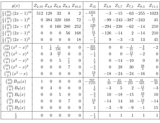
Table 1: Relations among double zeta values of weight 12 coming from Proposition 4. Each row of the table gives a relation among the (formal) double zeta values displayed in the top line. The

Z1,11column has been omitted, since all of its entries would be zero.

g(x) Z2,10Z4,8 Z6,6 Z8,4Z10,2 Z12 Z3,9 Z5,7 Z7,5 Z9,3 Z11,1 1

2 10 10

(2x−1)¹⁰ 512 128 32 8 2 −¹³⁵⁵₄ −3 −15 −63−255−1023

1 2

10 8

(2x−1)⁸ 0 384 320 168 72 −²¹₄ −99−243−387−243 45

1 2

10 6

(2x−1)⁶ 0 0 160 280 252 ¹²⁹₂ −294−238 −62 −14 210

1 2

10 4

(2x−1)⁴ 0 0 0 56 168 ⁵¹₂ −126 −14 2 −14 210

1 2

10 2

(2x−1)² 0 0 0 0 18 −⁷₄ 9 −3 −3 13 45

10 10

(x²−x)⁵ 1 ¹₆ ₁₂₆¹ 0 0 −³³¹₅₀₄ 0 0 −₂₁¹ −⁴₉ −2

10 8

(x²−x)⁴ 0 3 ¹⁰₇ 0 0 −¹₄ 0 0 −¹⁵₇ −2 0

10 6

(x²−x)³ 0 0 5 ⁷₂ 0 ¹₂ 0 −14 −10 0 0

10 4

(x²−x)² 0 0 0 7 0 −⁴₃ 0 28 30 ²⁸₃ 0

10 2

(x²−x) 0 0 0 0 9 ¹⁹₄ −18 −24 −24 −16 0

10 10

B10(x) 1 0 0 0 0 −₁₁₅₅⁷⁶⁷ ₃₃⁵ −₁₆₅⁴¹ −₂₃₁³¹ −₁₆₅⁴¹ −₃₃⁶¹

10 8

B8(x) 0 3 0 0 0 ¹₆ −3 5 2 −¹¹₃ −3

10 6

B6(x) 0 0 5 0 0 −⁴₃ 10 −18 −15 ¹⁶₃ 10

10 4

B4(x) 0 0 0 7 0 ¹³₆ −14 14 16 −¹⁴₃ −14

10 2

B2(x) 0 0 0 0 9 1 −3 −9 −9 −1 15

1

2 0 0 0 0 0 −¹₄ 1 1 1 1 1

and for the second basis we find 1

2 k−2

r−1

ar,s=











ν s−ν−1

(r, seven), (−1)^ν

k−2−2ν r−ν−1

− ν

r−ν−1

(r, sodd)

(we omit the value of λ in this case). In both cases, the coefficients for r, s even form a triangular matrix. The third family g(x) = B2ν(x) yields Eq. (7), as the reader can check as an exercise by imitating the proof of Eq. (5) which was given at the end of Section 3. The following table gives these three collections of relations for the case k= 12.

5. Double zeta values and period polynomials

In this section we describe various connections between period polynomials and the (formal) double zeta space, and prove Theorems 3 and 4. Since both of them involve period polynomials, we begin by reviewing these. The definition of period polynomials was already given briefly in the Introduction. The motivation comes from the connection with modular forms, which we will review in the next section.

Here we discuss only the algebraic properties.

The spaceWk is defined as

Wk = Ker(1 +S)∩Ker(1 +U+U²) ⊂Vk, (39) i.e. as the intersection of the (−1)-eigenspace of the involution S and the sum of the ⁻¹^±₂^√⁻³

-eigenspaces of the element U of order 3. Since εSε = S and

(14)

εU ε=U², the involutionεacts onWk and splits it as the direct sum of subspaces W_k^± = Wk ∩V_k^± of symmetric and antisymmetric polynomials. Since elements in Wk are also (−1)-eigenfunctions of S and since Sε = εS = δ, we also have W_k⁺ =W_k^od ⊂ V_k^+,od and W_k⁻ = W_k^ev ⊂ V_k^−,ev. Another important property of period polynomials is given by the following lemma.

Lemma. Letk >2be even. Then

Wk = Ker 1−T −T⁰, Vk and

W_k^± = Ker 1−T∓T ε, Vk

.

Proof. It is equivalent forf ∈Vk to be in Ker(1−T−T⁰) or to satisfyf|(1 +S) = f|(1+U+U²), since (1−T−T⁰)S= (1+S)−(1+U+U²). But a polynomial which is fixed by bothSandU is fixed by the full modular group and thus vanishes. The second assertion of the lemma follows from the first, because iff is annihilated by 1−T−T⁰ = 1−T−εT εandf|ε=±f thenf is also annihilated by 1−T∓T ε, and conversely if f is annihilated by 1−T ∓T ε then f = f|T(1±ε)∈ V_k^± and hencef|(1−T −T⁰) =f|(1−T−εT ε) = 0.

Remark. The operatorL= 1−T−T⁰plays a key role in the discovery by J. Lewis that there are holomorphic functions annihilated by this operator which have the same relation to the so-called Maass wave forms as period polynomials have to holomorphic modular forms ([10], [11]). We call the equation f|L = 0 the Lewis equation.

As in the Introduction, we denote byPk the subspace ofDk spanned by thePr,s

(andZk, but it can be omitted by virtue of Theorem 1), and byP_kêvthe subspace spanned by thePev,ev. Note that P_kêv corresponds to generating functions in V_kôd because of the shift by 1 in the exponents of X andY.

Theorem 3. The spacesP_k^ev and W_k⁻ are canonically isomorphic to each other.

More precisely, to each p ∈ W_k⁻ we associate the coefficients pr,s and qr,s (r+ s=k)which are defined by p(X, Y) =P k−2

r−1

pr,sX^r⁻¹Y^s⁻¹ andp(X+Y, Y) = P k−2

r−1

qr,sX^r⁻¹Y^s⁻¹. Then qr,s −qs,r = pr,s (in particular qr,s = qs,r for r, s even) and

X

r+s=k r, seven

qr,sZr,s ≡ 3 X

r+s=k r, s odd

qr,sZr,s (modZk), (40) and conversely, an element P

r, s oddcr,sZr,s ∈ Dk belongs to P_k^ev if and only if cr,s=qr,s arising in this way.

Remarks. 1. The equivalence of the first and last statements of the theorem follows from Theorem 2 : since the Zod,od form a basis of Dk, it is equivalent to speak of elements ofP_k^evor of relations of the form P(∗)Pev,ev=P(∗)Zod,od.

2. Since the double zeta realizations ζ(r)ζ(s) and ζ(k) of Pr,s (r, s even) and Zk are rational multiples ofπ^k, and since π^k is aQ-linear combination ofZod,od’s by Theorem 1, Theorem 3 as stated here contains the “rough statement” given in the Introduction. (The number of relations drops from dimW_k⁻ = dimMk to dimSk = dimMk−1 because one relation gets used up to eliminateζ(k).) Example 1. For every even k >2, the spaceW_k⁻ contains the polynomial p(x) = x^k⁻²−1 (in the inhomogeneous notation). Here p(x+ 1) =P

r6=1 k−2 r−1

x^r⁻¹, i.e., q1,k−1 = 0 and all other qr,s are equal to 1, and Theorem 3 reduces to a weaker version of Theorem 1.

(15)

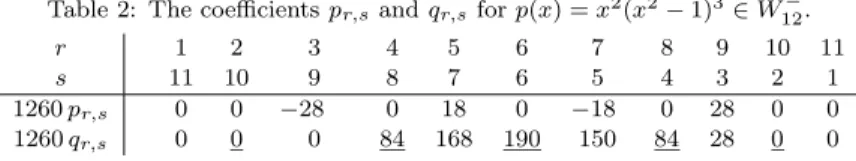
Table 2: The coefficientspr,sandqr,sforp(x) =x²(x²−1)³∈W₁₂⁻.

r 1 2 3 4 5 6 7 8 9 10 11

s 11 10 9 8 7 6 5 4 3 2 1

1260pr,s 0 0 −28 0 18 0 −18 0 28 0 0

1260qr,s 0 0 0 84 168 190 150 84 28 0 0

Example 2. The space W₁₂⁻ is 2-dimensional, spanned by the two polynomials p(x) =x¹⁰−1 andx²(x²−1)³. For the latter, we havep(x+ 1) =x⁸+ 8x⁷+ 25x⁶+ 38x⁵+ 28x⁴+ 8x³, so thepr,sandqr,sof the theorem are given (after multiplication by 1260) by the table

Theqr,swithrandseven (underlined) are symmetric and the relation (40), divided by 3, becomes

28Z8,4+190

3 Z6,6+ 28Z4,8≡28Z9,3+ 150Z7,5+ 168Z5,7 (modZ12), in agreement with Eq. (9) of the Introduction. The example fork= 16 given there arises in the same way from the polynomialp(x) =x²(x²−1)³(2x⁴−x²+ 2)∈W₁₆⁻. Proof. The function q = p|T satisfies q|(1−ε) = p|(T −T ε) = p|(T +εT ε) = p because p is antisymmetric and satisfies the Lewis equation. This shows that qr,s −qs,r = pr,s and also means that if we decompose q in the obvious way as q=qêv,++qêv,⁻+qôd,++qôd,⁻, thenqêv,⁻=¹₂pandqôd,⁻= 0. Write [a, b, c] to denoteaqêv,++bqêv,⁻+cqôd,+. Then

[0,2,0]T⁰ = p|T⁰ = p|εT ε = −p|T ε = −q|ε = [−1,1,−1], [1,−1,−1]T⁰ = q|ST⁰ = p|T ST⁰ = p|S=−p = [0,−2,0], and hence

[2,0,−2](T⁰−1) = [−1,−3,−1]− [2,0,−2] = [−3,−3,1].

This says that qôd−3qêv is the image under T⁰−1 of the symmetric polynomial 2 qêv,+−qôd,+

, so Proposition 2 implies Eq. (40). (The omitted coefficient ofZkin (40) is easily determined, by computing the integral in (31), asP

(−1)^r⁻¹qr,s.) This gives a mapW_k⁻−→ P_k^evwhich is obviously injective since the antisymmetrization of the coefficients on the right-hand side of (40) are the coefficients of p itself.

We omit the proof of surjectivity since it will follow from Theorem 4 below that dimW_k⁻= dimP_k^ev, so that injectivity suffices.

Theorem 3 tells us that, givenanyrelation of the form (29) inDkwithar,s=as,r

for r and s even, there exists a unique element p ∈ W_k⁻ such that the ar,s with r, s odd are equal to the numbersqr,s in the theorem. On the other hand, given an element of P_k^ev, its representation as a linear relation of the generatorsPev,ev

is not unique, because these generators are not linearly independent. The next proposition, which is a first form of Theorem 4 of the Introduction, describes the relations among them, i.e., all relations of the form (29) with ar,s = as,r for all r and s. It turns out that in any such relation the odd-index ar,s all vanish (in accordance with the widely believed and numerically verified statement that there are no relations overQamong products of values of the Riemann zeta function at odd arguments), while the even-index ar,s are related to the spaceW_k⁺.

Proposition 4. Let ar,s and µ be numbers with as,r =ar,s. Then the following three statements are equivalent:

(i) The relation

X

r+s=k

ar,sPr,s =µZk (41)

holds inDk.