数値解析の視線と立場

数値解析の視線と立場

齊藤 宣一

東京大学大学院数理科学研究科

新たな大学院教育の展開のためのFD研修会

—数値解析と量子コンピュータ— 大阪市立大学大学院理学研究科

2012年1月26日

大阪市立大学学術情報総合センター

自己紹介

氏名（しめい）：齊藤宣一（さいとう のりかず）

専門：偏微分方程式の数値解析

有限要素法，有限体積法，差分法の数学的基礎理論 仮想領域法，領域分割法の数学的基礎理論

走化性粘菌方程式(Keller-Segel系)，Navier-Stokes方程式など 解析半群，非線形半群によるアプローチ

非線形境界条件と解の正則性 経歴：

自己紹介

氏名（しめい）：齊藤宣一（さいとう のりかず）

専門：偏微分方程式の数値解析

有限要素法，有限体積法，差分法の数学的基礎理論 仮想領域法，領域分割法の数学的基礎理論

走化性粘菌方程式(Keller-Segel系)，Navier-Stokes方程式など 解析半群，非線形半群によるアプローチ

非線形境界条件と解の正則性 経歴：

明治大学理工学部数学科(B:1991∼1995, M:1995∼1997, D:1997∼1999) 博士(_理学)_{明治大学（}1999_年3月，指導教授： 藤田宏 教授）

（財）国際高等研究所(IIAS) 特別研究員 （1999∼2001）

富山大学教育学部・人間発達科学部（講師・助教授・准教授：2001∼2007） 東京大学大学院数理科学研究科（准教授：2007∼_）

目次

1

数値解析の立場；偏微分方程式の解析方法

2

数値解析の立場；コンピュータシミュレーションへの寄与

3

数値解析の教育（東大数理を例に）

4

学生・院生時代を振り返る

目次

1

数値解析の立場；偏微分方程式の解析方法

2

数値解析の立場；コンピュータシミュレーションへの寄与

3

数値解析の教育（東大数理を例に）

4

学生・院生時代を振り返る

数値解析

コンピュータを使った数学

数値解析研究者

コンピュータの達人

偏微分方程式の数値解析の立場から

無限次元を有限次元へ射影（離散化）

無限桁を有限桁で近似（コンピュータ）

目次

1

数値解析の立場；偏微分方程式の解析方法

2

数値解析の立場；コンピュータシミュレーションへの寄与

3

数値解析の教育（東大数理を例に）

4

学生・院生時代を振り返る

数値解析

コンピュータを使った数学

数値解析研究者

コンピュータの達人

偏微分方程式の数値解析の立場から

無限次元を有限次元へ射影（離散化）

無限桁を有限桁で近似（コンピュータ）

お詫び：“

理学部数学科

の立場で話します

§ 1. 数値解析の立場；偏微分方程式の解析方法

Keller-Segel _{の走化性モデル}

E. F. Keller & L. A. Segel (1970)

u=u(x,t): the cell density of the slime molds;

v =v(x,t): the concentration of the chemical substance;

∇ϕ(v): the velocity of udue tochemotaxis.

u Diffusion

f(v)

u u u

Chemotaxis

u v

f(v)

Creation of field

Keller-Segel system:

ut = −∇ ·j=∇ ·(Du∇u−u∇ϕ(v)) kvt = Dv∆v+g(u,v)

Motivation

1 u

が

集中化を相当におこしても，安定に計算を遂行できる数

値計算スキームの提案

2

解の正値性や質量の保存やエネルギーの散逸性を再現

なぜ必要か？

3

理論的な裏付け

なぜ必要か？

注意:

E. Nakaguchi and Y. Yagi (Hokkaido Math. J. 2002), A. Chertock and A.

Kurganov (Numer. Math. 2008), Y. Epshteyn and A. Izmirlioglu (J. Sci. Comput.

2009), (SIAM J. Numer. Anal. 2008/09)

J. Haˇskovec and C. Schmeiser (J. Stat. Phys. 2009).

F. Filbet (Numer. Math. 2006)finite volume

S (IMA J. Numer. Anal. 2007), (RIMS Bessatsu 2009), (CPAA 2012)

conservative finite element

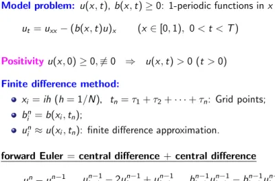
Illustration of the issue

Model problem: u(x,t),b(x,t)≥0: 1-periodic functions inx ut=uxx−(b(x,t)u)x (x∈[0,1), 0<t<T)

Positivityu(x,0)≥0,6≡0 ⇒ u(x,t)>0 (t >0) Finite difference method:

xi=ih (h= 1/N)，tn=τ1+τ2+· · ·+τn: Grid points;

bⁿ_i =b(xi,tn);

uⁿ_i ≈u(xi,tn): finite difference approximation.

forward Euler=central difference +central difference u_iⁿ−uⁿ_i⁻¹

τn

=u_i−1ⁿ⁻¹−2uⁿ⁻¹_i +uⁿ⁻¹_i+1

h² −bⁿ⁻¹_i+1u_i+1ⁿ⁻¹−bⁿ⁻¹_i−1u_i−1ⁿ⁻¹ 2h

Numerical example

b(x,t) = 4(1 + cos 2πx)(1 +t)²

，h

，τ

0 0.2

0.4 0.6

0.8

0 0.5 1 1.5 2 2.5 3 3.5 4 0

2 4

0≤tn≤4.0

Numerical example

b(x,t) = 4(1 + cos 2πx)(1 +t)²

，h

，τ

0 0.2

0.4 0.6

0.8

1 0 0.5 1 1.5 2 2.5 3 3.5 4 4.5 -8

-4 0 4 8

0≤tn≤4.4

Numerical example

b(x,t) = 4(1 + cos 2πx)(1 +t)²

，h

，τ

0 0.2

0.4 0.6

0.8

1 4.37 4.375

4.38 4.385

4.39

4.395 4.4 -80

-40 0 40 80

4.37≤tn≤4.4

Numerical example

b(x,t) = 4(1 + cos 2πx)(1 +t)²

，h

，τ

-50 -40 -30 -20 -10 0 10 20 30 40 50

0 0.2 0.4 0.6 0.8 1

u-axis

x-axis

4.37≤tn≤4.4 (another view-point)

Consideration

Finite difference scheme λn=τn/h²

⇔ uⁿi = (1−2λn)uⁿ⁻¹_i +

λn+ τn

2hbⁿ⁻¹_i−1

uⁿ⁻¹_i−1 + λn−τn

2hb_i+1ⁿ⁻¹ uⁿ⁻¹_i+1

Non-negativity (*) u_iⁿ⁻¹≥0 (∀i) ⇒ u_iⁿ≥0 (∀i) A sufficient condition:

(· · ·)≥0，(· · ·)≥0，(· · ·)≥0⇒(*) h≤ 1

2βⁿ⁻¹ ⇒(*).

βⁿ= max

1≤i≤Nbⁿi

Before computation, we have to choosehsatisfying:

h≤ 1 2βT

, βT = max

0≤tn≤Tβⁿ.

Upwind finite difference scheme

forward Euler=central difference

＋

τn

=u_i−1ⁿ⁻¹−2uⁿ⁻¹_i +uⁿ⁻¹_i+1

h² −bⁿ⁻¹_i u_iⁿ⁻¹−bⁿ⁻¹_i−1u_i−1ⁿ⁻¹ h

⇔

uⁿi =

1−2λn−τn

hb_iⁿ⁻¹

u_iⁿ⁻¹+ λn+τn

hbⁿ⁻¹_i−1

uⁿ⁻¹_i−1 +λnu_i+1ⁿ⁻¹

A sufficient condition： τn≤ h²

2 +hβn−1 ⇒(*).

In each time step, were-chooseτnto satisfy the above condition.

Extension tod≥2 and arbitrary Ω

FEM; Tabata (1977), Heinrich et al. (1977)→flow problems.

In general, the upwind FEM destroys theconservation of mass.

Conservative numerical schemes;

FEM; Baba-Tabata upwinding (1981), Finite volume method (FVM), ....

Upwind finite difference scheme

forward Euler=central difference

＋

τn

=u_i−1ⁿ⁻¹−2uⁿ⁻¹_i +uⁿ⁻¹_i+1

h² −bⁿ⁻¹_i u_iⁿ⁻¹−bⁿ⁻¹_i−1u_i−1ⁿ⁻¹ h

⇔

uⁿi =

1−2λn−τn

hb_iⁿ⁻¹

u_iⁿ⁻¹+ λn+τn

hbⁿ⁻¹_i−1

uⁿ⁻¹_i−1 +λnu_i+1ⁿ⁻¹

A sufficient condition： τn≤ h²

2 +hβn−1 ⇒(*).

In each time step, were-chooseτnto satisfy the above condition.

Extension tod≥2 and arbitrary Ω

FEM; Tabata (1977), Heinrich et al. (1977)→flow problems.

In general, the upwind FEM destroys theconservation of mass.

Conservative numerical schemes;

FEM; Baba-Tabata upwinding (1981), Finite volume method (FVM), ....

主テーマ

に対する保存的スキームの開発と解析

§ 2. 数値解析の立場；コンピュータシミュレーションへ

の寄与

CREST: 放射線医学と数理科学の協働による高度臨床診 断の実現

http://www.ems.okayama-u.ac.jp/suito/CREST/index.html

代表者：水藤寛（岡山大学，応用数学，数値流体力学）

共同研究者：植田琢也（聖路加国際病院，放射線科医師），栗原考次（岡山

大学，統計学），滝沢研二（早稲田大学高等研究所，数値流体力学），齊藤

数学の役割

-

? 6

対象 数理モデル

(

微分方程式

計算モデル

@@

@@

@@

@@

@@

@@

@

@ I

@@

@@

@@

@@

@@

@@R

verification validiation

Boundary conditions for the NS equations

In a domain Ω⊂R^d, we consider

∂u

∂t + (u· ∇)u=ν∆u− ∇p+f, ∇ ·u= 0.

On the boundary∂Ω, we usually pose:

Dirichlet condition (adhesive condition)u=β with R

∂Ωβ ds= 0;

Slip condition (Navier’s condition)un= 0 and στ(u) = 0;

Penetration conditionuτ= 0 and σn(u,p) = 0.

Notation.

n: the outer unit normal to the boundary;

For vector fieldu, setun=u·nanduτ=u−nun; ei,j(u) = 1

2 ∂ui

∂xj

+∂uj

∂xi

: the rate-of-strain tensor foru;

Ti,j(u,p) =−pδij+ 2νei,j(u): Cauchy stress tensor;

σ(u,p) = (Tij(u,p))n=nσn(u,p) +στ(u): the stress (traction) vector.

Slip boundary condition of friction type

For given amodulus function of frictiong =g(s) (s∈∂Ω), on∂Ω:

(i)







|στ(u)|<g ⇒ uτ = 0,

|στ(u)|=g ⇒

( uτ= 0 oruτ 6= 0,

uτ6= 0⇒στ(u) =−guτ/|uτ|

⇔(ii)|στ(u)| ≤g, στ(u)·uτ+g|uτ|= 0;

⇔(iii)un= 0, −στ(u)∈g∂|uτ|.

It was proposed by H. Fujita (1994) in order to model some flow phenomena in applications (flow through a drain with its bottom covered by sherbet, and so on....). He studied weak solutions of the stationary Stokes and NS equations.

A similar condition is well studied in contact problems of the elasticity theory.

Notation (subdifferential). Forz ∈R^m,

∂|z|=

(z/|z| (z 6= 0) {w ∈R^m| |w| ≤1} (z = 0).

Leak boundary condition of friction type

For given amodulus function of frictiong =g(s) (s∈∂Ω), on∂Ω:

(i)







|σn(u,p)|<g ⇒ un= 0,

|σn(u,p)|=g ⇒

un= 0 orun6= 0,

un6= 0⇒σn(u,p) =−gun/|un|

⇔(ii)|σn(u,p)| ≤g, σn(u,p)un+g|un|= 0;

⇔(iii)uτ = 0, −σn(u,p)∈g∂|un|.

It was also proposed by H. Fujita (1994) in order to model some flow phenomena in applications (flow through a certain filter with semi-permeable membrane, and so on....).

The motivation of introducing those BC comes from practical intention to model mathematically certain flow phenomena in applications.

On the other hand, the study of those BC deserves theoretical interests for its own sake because of the coherent use of celebrated methods in applied analysis. Also, they bring us somenew methodsandtools(from both analytical and numerical viewpoints) to attack some flow phenomena.

Applications

Some successful applications by Prof. Suito’s group:

1 Wave motion breaking on the shore (environmental problem)

2 Pollution due to spilled oil into the sea (environmental problem)

3 Cerebrospinal fluid flow problem (medical problem)

The Stokes problem with the leak BC of friction type

(S-LF)

Findu= (u1, . . . ,ud) : Ω→R^d andp: Ω→Rs.t.







−ν∆u+∇p=f, ∇ ·u= 0 in Ω,

u= 0 on Γ0,

uτ= 0, −σn∈g∂|un| on Γ1

Ω⊂R^d: b’dd domain (d= 2,3), ∂Ω = Γ0∪Γ1; f ∈L²(Ω)^d; 0<g∈L^∞(Γ1); ν >0.

Remark. BC on Γ1may be replaced by either (i)|σn| ≤g, σnun+g|un|= 0 or

(ii) 8

<

:

|σn|<g =⇒ un= 0,

|σn|=g =⇒

 un= 0 orun6= 0,

un6= 0 =⇒σn=−gun/|un| G W G

0 1

Variational formulation: variational inequality

For anyv∈Kτ ={v ∈H¹(Ω)^d |v = 0 on Γ0, vτ = 0 on Γ1}, we have:

Z

Γ1

σnvn dS= 2ν Z

Ω

eij(u)eij(v)dx

| {z }

=a(u,v)

− Z

Ω

p(∇ ·v)dx

| {z }

=b(v,p)

− Z

Ω

fv dx

| {z }

=(f,v)

,

Z

Γ1

g|vn|dS

| {z }

=j(vn)

− Z

Γ1

g|un|dS ≥ − Z

Γ1

σn(vn−un)dS.

(W-S-LF)

Find (u,p)∈Kτ×L²(Ω) s.t.







a(u,v−u) +b(v−u,p) +j(vn)−j(un)≥(f,v−u) (∀v∈Kτ),

b(u,q) = 0 (∀q∈L²(Ω))

A issue on non-uniqueness of p

Let (u,p^∗) be a solution of (W-S-LF) and set k1= sup

Γ1

[σn(u,p^∗)−g], k2= inf

Γ1

[σn(u,p^∗) +g].

Then,p=p^∗+k, withk∈[k1,k2], is also an associating pressure ofu.

un6= 0 on Γ⁰₁⊂Γ1⇒pis uniquely determined.

Example. We consider

Ω ={(r, θ)| 1<r<2}, Γ0={r= 1}, Γ1={r= 2}.

Then, the functionsu(r, θ) =w(r)e^θ andp(r) =κr solve

−∆u+∇p=−6eθr⁻²+κer, ∇ ·u= 0 in Ω, u|Γ0= 0, u^τ|Γ1= 0, un|Γ1= 0, σn(u,p) =−p(r), |σn(u,p)|= 2κ, wherew(r) = 4r⁻¹+ 2r−6 andκ >0 is a constant.

Setg= 2κ+ 1. (u,p) above is a solution of (W-S-LF). Moreover,

 k∈[k1,k2] = [−1−4κ,1] ⇒ (u,p+k) solves (W-S-LF);

k6∈[k1,k2] ⇒ (u,p+k) does not solve (W-S-LF).

(Notice thatk6∈[k1,k2]⇒ |σn(u,pk)|>g.)

Triangulation

Below Ω is assumed to be a polygon and Γ1is a side of∂Ω and Γ0=∂Ω\Γ1. {T_h}^hfamily of regular triangulations of Ω.

Nodes on Γ1are numbered asM1,M1/2,M2, . . . ,Mm and set Γ1,h = {M1,M1/2,M2, . . . ,Mm+1/2,Mm},

Γ⁰_1,h = {M1/2,M2, . . . ,Mm+1/2}.

Similarly, Γ0,h denotes the set of all nodes locating on Γ0. The P2/P1 finite element spaces:

Vh = {v ∈C(Ω)²|v|^T ∈P₂(∀T ∈T_h)},

Vhτ = {v ∈Vh|v(M) = 0 (∀M∈Γ0,h), vτ(M) = 0 (∀M ∈Γ⁰_1,h)}, Qh = {q∈C(Ω)|q|^T ∈P₁ (∀T ∈T_h)}.

Finite element approximation (W-S-LFh)

(W-S-LFh)

Find (uh,ph)∈Vhτ×Qh s.t.











a(uh,vh−uh) +b(vh−uh,ph)

+jh(vhn)−jh(uhn)≥(f,vh−uh) (∀vh∈Vhτ),

b(uh,qh) = 0 (∀qh∈Qh)

Here, the barrier term of frictionj(η) is approximated by

jh(η) = 1 6

Xm

i=1

|ei| gi|ηi|+ 4gi+1/2|ηi+1/2|+gi+1|ηi+1| , wheregi+s =g(Mi+s),ηi+s =η(Mi+s) and ei = dist (Mi,Mi+1).

Error estimates under regularity assumptions

Forq∈L²(Ω), we write ˜p=p− |Ω|⁻¹(p,1)L².

Theorem 1 (Kashiwabara, 2009)

g∈C¹(Γ);

(u,p)∈H^1+ε(Ω)²×H^ε(Ω), for someε∈(0,2), solution of (W-S-LF).

(i) We have:

ku−uhk^H1+k˜p−˜phk^L2 ≤Chmin{ε/2,1/4}

(ii) Further, if p−ph∈L²₀(Ω), we have

ku−uhkH¹+kp−phkL² ≤Ch^min{ε,1/4}

Remark. Ifε= 2 is possible, we have onlyO(h^1/4), which is not the optimal rate of convergence of the P2 element.

Error estimates under regularity and sign conditions

Theorem 2 (Kashiwabara, 2009)

g∈C²(Γ); (u,p)∈H^1+ε(Ω)²×H¹(Ω) for someε∈(0,2).

p−ph∈L²₀(Ω); The sign condition is satisfied.

(i) We have:

ku−uhk^H1+kp−phk^L2 ≤Ch^min{ε,1}

(ii) Further, if g is a polynomial of the degree≤1, we have ku−uhk^H1+kp−phk^L2 ≤Ch^ε.

The sign condition

Solutionsuanduh of (W-S-LF) and (W-S-LFh) satisfy:

1 (Πhu)n anduhnhave zeros only at nodesM1,M2, . . . ,Mm+1 on Γ1;

2 sign (un) = sign ((Πhu)n) on Γ1.

Πh:C(Ω)→Vhdenotes the Lagrange interpolation operator.

Numerical examples

Geometry: Ω = (0,1)², Γ1={(x,1)|0<x <1}(Green), Γ0= Ω\Γ1

Data: ν= 1 and f1(x,y) = 0;

f2(x,y) = 120(2x−1)y²(1−y)²

+80x(1−x)(1−2x)(6y²−6y+ 1) + 8(6x⁵−15x⁴+ 10x³) If we poseu= 0 on Γ1, then (u,p) is given as

0 0.2 0.4 0.6 0.8 1

0 0.2 0.4 0.6 0.8 1

y

x u

0 0.2

0.4 0.6 0.8

1 0 0.2

0.4 0.6

0.8 1 -4

-3 -2 -1 0 1 2 3 4

x

y

p

Numerical examples (W-S-LFh)’

0 0.2 0.4 0.6 0.8 1

0 0.2 0.4 0.6 0.8 1

y

x

Figure: g = 0.1

0 0.2 0.4 0.6 0.8 1

0 0.2 0.4 0.6 0.8 1

y

x

Figure: g= 1.2

0 0.2 0.4 0.6 0.8 1

0 0.2 0.4 0.6 0.8 1

y

x

Figure: g= 3.0

Nonstationary NS with leak BC of friction type

(ENS-LF)

Findu: [0,T]×Ω→R^d andp: [0,T]×Ω→R:











ut−ν∆u+ (u· ∇)u+∇p=f, ∇ ·u= 0 in (0,T)×Ω,

u= 0 on (0,T)×Γ0,

uτ= 0, −σn∈g∂|un| on (0,T)×Γ1, u|^t=0=u0.

Ω⊂R^d: b’dd domain (d= 2,3), ∂Ω = Γ0∪Γ1

Nonstationary NS with leak BC of friction type

(W-ENS-LF)

Find, for a.e. t ∈(0,T), (u(t),p(t))∈Vτ×L²(Ω) s.t.











(u⁰,v−u) +a(u,v−u) +a1(u,u,v−u)

+b(v−u,p) +j(vn)−j(un)≥(f,v−u) (∀v∈Vτ),

b(u,q) = 0 (∀q∈L²(Ω)),

u(0) =u0. Here, as usual,

a1(u,v,w) = Z

Ω

[(u· ∇)v]·w dx. Difficulty.

a1(u,v,u) = 1 2 Z

Γ1

un|v|² dS (if∇ ·u= 0 in Ω, un= 0 on Γ0).

Nonstationary NS with leak BC of friction type

T. Kashiwabara has recently proved:

Theorem 3 (Kashiwabara, 2010)

Suppose that

1 Γ0: class of C²andΓ1: class of C⁴,

2 f ∈L^∞(0,T;L²(Ω)^d)and f⁰∈L²((0,T)×Ω)^d,

3 g∈H¹(0,T;L²(Γ1))and g(0)∈H¹(Γ1),

4 u0∈H²(Ω)^d∩Vτ satisfies the leak BC of friction type (with g(0)), and u0,n= 0onΓ1.

Then, for a suitably small0<T⁰ <T , there exists

(u∈L^∞(0,T⁰;Vτ), u⁰ ∈L^∞(0,T⁰;L²(Ω)^d)∩L²(0,T⁰;Vτ), p∈L^∞(0,T⁰;L²(Ω)^d)

satisfying (W-ENS-LF) in[0,T⁰].

個人的な思い

コンピュータ・シミュレーションによる諸現象の研究は，狭い意味での理工 学を超えて，生命科学，臨床医学，経済学にまで応用範囲を拡げ，広く有益 な情報をもたらしている．

複雑かつ大規模なコンピュータ・シミュレーションにおける数学的諸問題を 解決することは，数学の重要な役割の一つ．

実際，シミュレーションは，コンピュータの内部で完結するものではなく，

対象とする現象の数理モデル化，モデルの数学解析，近似と離散化，アルゴ

幹で強く繋がっている．

すなわち，数値解析は，数学的真理の追求と数学を通じた社会への貢献を両

立できる研究テーマ

§ 3. 数値解析の教育（東大数理を例に）

東大数理における数値解析関係の講義

1

計算数理

年，夏学期，金曜

限)

2

計算数理演習

年，夏学期，金曜

限)

3

計算数理

年・大学院，夏学期，木曜

限)

菊地文雄教授（現，一橋大学特任教授）

有限要素法の数学的理論のパイオニア

数値解析入門 (1/2)

計算数理

年)

1 浮動小数点数

2 連立一次方程式

直接法(Gaussの消去法，LU分解)，線形反復法(Jacobi法，Gauss-Seidel法，SOR法) ノルム，行列ノルム，条件数，安定性解析

3 補間と積分

Lagrange補間多項式と複合積分公式(中点則，台形則など) 直交多項式とGauss型積分公式

4 非線形方程式

Newton法，多次元Newton法， 縮小写像の原理と反復法の収束

5 常微分方程式の初期値問題

一段法の解析，Runge-Kutta法の構成，埋め込み型公式，絶対安定領域

6 共役勾配法(A:正定値対称)

二次形式J(x) = ¹₂x·Ax−b·xの最小化問題

Kryrov部分空間Kn(A,b) = span{b,Ab,A²b, . . . ,Aⁿ⁻¹b}の役割

数値解析入門 (2/2)

計算数理演習

年)

1 計算数理Iで扱った話題に関する計算実習

2 自作のプログラムで実習，結果をレポート(L^ATEX→pdf)で提出．

3 プログラミングの演習ではない．言語の選択は自由．

4 初心者向けに，ガイダンス(参考資料)，サンプルプログラム(C言語)を配布して，準備期間(1ヶ月間)を 設けている．

要点

算法の紹介とプログラミングが主眼ではない．

抽象的な数学理論が，具体的な算法の設計・解析にどのよう寄与するのかを理解してもらうことを目標．

“はじめての応用数学”

応用数学6=既成数学の適用の羅列.

実用価値の低い算法を取り上げることもある．

例題 1 _{：グラフ描画の問題} (?)

自然数

をパラメータとする関数

fN(x) = XN

m=1

4

(2m−1)πsin(2m−1)x (−π≤x≤π)

について，N

の時のグラフを描け．

例題 1 _{：グラフ描画の問題} (?)

自然数

をパラメータとする関数

fN(x) = XN

m=1

4

(2m−1)πsin(2m−1)x (−π≤x≤π)

について，N

の時のグラフを描け．

-1.5 -1 -0.5 0 0.5 1 1.5

-4 -3 -2 -1 0 1 2 3 4

(f1(x),f5(x),f20(x),f50(x))

-1.5 -1 -0.5 0 0.5 1 1.5

-4 -3 -2 -1 0 1 2 3 4

(f50(x)

のみ

例題 1 _{：グラフ描画の問題} (?)

自然数

をパラメータとする関数

fN(x) = XN

m=1

4

(2m−1)πsin(2m−1)x (−π≤x≤π)

について，N

の時のグラフを描け．

-1.5 -1 -0.5 0 0.5 1 1.5

-4 -3 -2 -1 0 1 2 3 4

(f1(x),f5(x),f20(x),f50(x))

-1.5 -1 -0.5 0 0.5 1 1.5

-4 -3 -2 -1 0 1 2 3 4

(f50(x)

のみ

ヒントと例題が命取り

次のようなヒントを付記した：何をして良いかわからない人には，

「教育用計算機システムにおける数値計算の第一歩: gnuplotの利用」と「C言語 一夜漬け」の第8章が参考になるでしょう．

nを与えて，x_i=ih，(i= 0, . . . ,n)，h=2π n として，

xiにおける関数値f(xi)のリスト

x0 f(x0) x1 f(x1)

.. .

.. . x_n f(xn)

を出力するプログラムを作成する．そして，

gnuplot(ニュープロット)でグラフを描画する．

そして，サンプルプログラムを数題載せたが，実行例で，

いずれもn= 100としてしまった．

しかし，いまの場合f50(x)を表現するのに，n= 100で は不足(n≥200が必要)．

これは，いろいろな意味で，良い教訓．

例題 2 _{：定積分の計算}

次の定積分を，等間隔標本点

を用いて，複合中 点則

で計算して，結果を検 討せよ．特に，小区間の長さ

と誤差の関係を詳しく調べよ．

Q(f) = Z 1

0

e^πxsin(πx)dx= e^π+ 1

2π , f(x) =e^πxsin(πx), Q(f) =

Z 1 0

p1−x²dx= π

4, f(x) =p

1−x² 定理.

f ∈C²[0,1] ⇒ |Q(f)−Rh(f)| ≤ 1

24h²kf⁰⁰k^L∞, f ∈C²[0,1] ⇒ |Q(f)−Th(f)| ≤ 1

12h²kf⁰⁰k^L∞, f ∈C⁴[0,1] ⇒ |Q(f)−Sh(f)| ≤ 1

2880h⁴kf⁽⁴⁾k^L∞

これらを，例えば，|

と書くのは良くない．

数値例の検討

E⁽¹⁾(f) =Q(f)−Rh(f)

などとおいて，

|Eh|=Ch^ρ ⇔ρ=log|Eh(f)|/log(Ch)

を仮定して，計算により

を推定．

h ρ⁽¹⁾_h ρ⁽²⁾_h ρ⁽³⁾_h 2⁻² 1.803 1.894 4.121 2⁻⁴ 1.990 1.994 4.010 2⁻⁶ 1.999 2.000 4.001 2⁻⁸ 2.000 2.000 4.000

f(x) =e^πxsin(πx)

h ρ⁽¹⁾_h ρ⁽²⁾_h ρ⁽³⁾_h 2⁻² 1.476 1.489 1.507 2⁻⁴ 1.494 1.497 1.502 2⁻⁶ 1.498 1.499 1.500 2⁻⁸ 1.500 1.500 1.500

f(x) =p 1−x² f(x) =√

1−x²

については，f

であるが，f

ではなく，

kf⁰⁰k^L∞ = +∞

となっているため，定理は適用できない

しかし，|

が予想できる

実際に，

が成り立つので，この仮定の下で，

|Rh(g)−Q(g)| ≤Ch^3/2kg⁰⁰k²

の形の誤差評価を導くことができる．

もっと緩い仮定の下での誤差評価

例題 3 ：常微分方程式の初期値問題

次の問題を，一様刻み幅

のホイン法，古典的ルンゲ・クッタ法

ふつうのル ンゲ・クッタ法)，ランベルト法

段数

次公式) で計算して，誤差の

へ依存 性を調べよ．

d

dtu(t) =− 1

2e^t−1u(t) (0<t <1), u(0) = 2, d

dtv(t) =v(t)[1−v(t)] (0<t<1), v(0) = 2

ルンゲ・クッタ法の復習

常微分方程式

dtu(t) =f(t,u(t)) (0<t<T), u(0) =a.

離散変数

ホイン法(2

段数

次精度のルンゲ・クッタ法)











Un+1=Un+h

2(k1+k2) k1=f(tn,Un)

k2=f (tn+h,Un+hk1).

誤差評価:

u∈C³[0,T] ⇒ max

0≤tn≤T|u(tn)−Un| ≤Ch².

ルンゲ・クッタ法の復習

常微分方程式

dtu(t) =f(t,u(t)) (0<t<T), u(0) =a.

離散変数

古典的ルンゲ・クッタ法(4

段数

次精度のルンゲ・クッタ法)



















Un+1=Un+h

6(k1+ 2k2+ 2k3+k4) k1=f(tn,Un)

k2=f tn+¹₂h,Un+¹₂hk1 k3=f tn+¹₂h,Un+¹₂hk2

k4=f (tn+h,Un+hk3)

誤差評価:

u∈C⁵[0,T] ⇒ max

0≤tn≤T|u(tn)−Un| ≤Ch⁴.

ルンゲ・クッタ法の復習

常微分方程式

dtu(t) =f(t,u(t)) (0<t<T), u(0) =a.

離散変数

，近似解

ランベルト法(4

段数

次精度のルンゲ・クッタ法)



















Un+1=Un+h

6(k1+ 4k2+k4) k1=f(tn,Un)

k2=f tn+¹₂h,Un+¹₂hk1 k3=f tn+¹₂h,Un+¹₂hk1−³2hk2 k4=f tn+h,Un+⁴₃hk2−¹3hk3

誤差評価:

u∈C⁵[0,T] ⇒ max

0≤tn≤T|u(tn)−Un| ≤Ch³.

数値例の検討

積分のときと同様に，E

0≤tn≤T|u(tn)−Un|

とおいて，E

を仮定し て，ρ の値を推定．

h ρ⁽¹⁾_h ρ⁽²⁾_h ρ⁽³⁾_h 0.05000 2.053 4.044 3.248 0.02500 2.028 4.025 3.126 0.01250 2.014 4.014 3.063 0.00625 2.007 4.007 3.031

h ρ⁽¹⁾_h ρ⁽²⁾_h ρ⁽³⁾_h 0.05000 2.082 4.028 4.023 0.02500 2.048 4.023 4.023 0.01250 2.024 4.014 4.012 0.00625 2.012 4.007 4.007

ランベルト法は，自励系に対しては

次精度となる

次精度)．

数値例の検討

積分のときと同様に，E

0≤tn≤T|u(tn)−Un|

とおいて，E

を仮定し て，ρ の値を推定．

h ρ⁽¹⁾_h ρ⁽²⁾_h ρ⁽³⁾_h 0.05000 2.053 4.044 3.248 0.02500 2.028 4.025 3.126 0.01250 2.014 4.014 3.063 0.00625 2.007 4.007 3.031

h ρ⁽¹⁾_h ρ⁽²⁾_h ρ⁽³⁾_h 0.05000 2.082 4.028 4.023 0.02500 2.048 4.023 4.023 0.01250 2.024 4.014 4.012 0.00625 2.012 4.007 4.007

ランベルト法は，自励系に対しては

次精度となる

次精度)．

もう一度，方程式を見てみる：

d

dtu(t) =− 1

2e^t−1u(t) (0<t <1), u(0) = 2, d

dtv(t) =v(t)[1−v(t)] (0<t<1), v(0) = 2

数値例の検討

積分のときと同様に，E

0≤tn≤T|u(tn)−Un|

とおいて，E

を仮定し て，ρ の値を推定．

h ρ⁽¹⁾_h ρ⁽²⁾_h ρ⁽³⁾_h 0.05000 2.053 4.044 3.248 0.02500 2.028 4.025 3.126 0.01250 2.014 4.014 3.063 0.00625 2.007 4.007 3.031

h ρ⁽¹⁾_h ρ⁽²⁾_h ρ⁽³⁾_h 0.05000 2.082 4.028 4.023 0.02500 2.048 4.023 4.023 0.01250 2.024 4.014 4.012 0.00625 2.012 4.007 4.007

ランベルト法は，自励系に対しては

次精度となる

次精度)．

もう一度，方程式を見てみる：

d

dtu(t) =− 1

2e^t−1u(t) (0<t <1), u(0) = 2, d

dtv(t) =v(t)[1−v(t)] (0<t<1), v(0) = 2

厳密解

．

例題 4 _{：単振動の方程式}

単振動の方程式：−

dt²x(t) =x(t)

一般解：x

定数)

初期条件

の下で数値計算．

教科書には、、、

d

dtu(t) =f(u(t)), u= u1

u2

= x

x⁰

, f(u) = u2

−u1

−→Runge-Kutta

法など、、、、t

0≤maxt_n≤Tku(tn)−Uⁿk∞≤CTh⁴.

Runge-Kutta _{法による計算例}

-1 -0.5 0 0.5 1

0 2 4 6 8 10

x(t) = cost+Bsint

-1 -0.5 0 0.5 1

0 5 10 15 20 25 30

05t 530

-1 -0.5 0 0.5 1

0 2 4 6 8 10

05t 510

-1 -0.5 0 0.5 1

0 20 40 60 80 100

05t 5100

別の解法：差分法

微分方程式の近似を考える上で，差分法は最も基本的．

前進差分

dt ≈x(t+h)−x(t)

h

， 後退差分

dt ≈x(t)−x(t−h) h

二階中心差分

dt² ≈ x(t−h)−2x(t) +x(t+t) h²

−x⁰⁰(t) =x(t)

，

，

は，より自然に

−Xn−1−2Xn+Xn+1

h² =Xn (n≥1), X⁰= 0, X¹−X⁰

h =B

と近似できる．ただし，X

であり，

0≤tmaxn≤T|x(tn)−Xⁿ| ≤CTh (O(h²)

ではない！)

差分法と Runge-Kutta _法の比較

-1 -0.5 0 0.5 1

0 2 4 6 8 10

x(t) = cost+Bsint

-1 -0.5 0 0.5 1

0 2 4 6 8 10

x(t) = cost+Bsint

(いずれも，h= 1)

差分法と Runge-Kutta _法の比較

-1 -0.5 0 0.5 1

0 2 4 6 8 10

差分法

-1 -0.5 0 0.5 1

0 2 4 6 8 10

Runge-Kutta

法

(いずれも，h= 1)

差分法と Runge-Kutta _法の比較

-1 -0.5 0 0.5 1

0 5 10 15 20 25 30

差分法

-1 -0.5 0 0.5 1

0 5 10 15 20 25 30

Runge-Kutta

法

(いずれも，h= 1)

差分法と Runge-Kutta _法の比較

-1 -0.5 0 0.5 1

0 20 40 60 80 100

差分法

-1 -0.5 0 0.5 1

0 20 40 60 80 100

Runge-Kutta

法

(いずれも，h= 1)

エネルギーの保存

単振動の方程式の解

E = dx

dt 2

+x²= Const.

差分法の解

h 2

+Xⁿ⁺¹Xⁿ= Const.

Runge-Kutta

法の解

· · · ·?

ここからの教訓、、、、目的や，数学的な仮定・前提を意識することが重要

偏微分方程式の数値解析

計算数理

数学科

年，夏学期

1 熱方程式(1D)に対する差分近似

2 反応拡散系(1D)に対する差分近似

3 Poisson方程式(2D)に対する有限要素法

4 Lax-Milgramの理論

要点

算法の紹介が主眼ではない．

関数解析（特に，ソボレフ空間）の一部の定理を除いて，self-contained に 行う．

深刻な問題点：演習の時間がない．仮にあったとしても，有限要素法のプロ グラムは敷居が高い．

→freefem++cs

の利用は有効

FreeFem++

J. L. Lions

数値解析研究所

FreeFem++ team(O. Pironneau, F. Hecht, A. Le Hyaric, J. Morice) http://www.freefem.org/ff++/

統合環境FreeFem++cs

http://www.ann.jussieu.fr/^∼lehyaric/ffcs/index.htm

例題： − ∆u(x , y ) = f (x , y ) in Ω with u |

= 0

Poisson方程式の弱形式: Findu∈V =H¹₀(Ω) satisfying

J(u,v) = ZZ

Ω

∇u(x,y)· ∇v(x,y)dxdy− ZZ

Ω

f(x,y)v(x,y)dxdy= 0 (∀v∈V)

func g = 0;

func f = 1 - y*x^2;

int n = 40;

border G1(t = 0, 2*pi) { x = 2*cos(t); y = sin(t); } mesh Th = buildmesh(G1(n));

fespace Vh(Th,P1);

Vh u,v;

solve poisson (u,v) =

int2d(Th)(dx(u)*dx(v) + dy(u)*dy(v)) - int2d(Th)(f*v) + on(G1, u = g);

plot(u, ps="example1.eps");

応用：非線形楕円型偏微分方程式の解

有界領域

で，非線形楕円型方程式

−∆u=u^p, u≥0 in Ω, u= 0 on∂Ω, p>1.

Nehari

の解

u∈V =H₀¹(Ω), J(u) = inf

v∈NJ(v).

ただし，

J(v) = ZZ

Ω

1

2|∇v|²− 1

p+ 1|v|^p+1

dxdy, N =

v ∈V

ZZ

Ω|∇v|²dxdy = ZZ

Ω|v|^p+1dxdy >0

数値計算例： p = 3

0 0.5 1 1.5 2 2.5 3 3.5 4 4.5 5

0 0.5

1 1.5

2 2.5

3 0 0.5 1 1.5 2 2.5 3

0 0.5 1 1.5 2 2.5 3 3.5 4 4.5 5

0 1 2 3 4 5 6

0 0.5

1 1.5

2 2.5

3 0 0.5 1 1.5 2 2.5 3

0 1 2 3 4 5 6

0 0.5 1 1.5 2 2.5 3 3.5 4 4.5 5

0 0.5

1 1.5

2 2.5

3 0 0.5 1 1.5 2 2.5 3

0 0.5 1 1.5 2 2.5 3 3.5 4 4.5 5

数値計算例： p = 3 ( _{スケーリング反復法} )

0 1 2 3 4 5 6 7 8

0 0.5

1 1.5

2 2.5

3 0 0.5 1 1.5 2 2.5 3

0 1 2 3 4 5 6 7 8

x

y

-1 0 1 2 3 4 5 6 7 8

0 0.5

1 1.5

2 2.5

3 0 0.5 1 1.5 2 2.5 3

-1 0 1 2 3 4 5 6 7 8

x

y

0 1 2 3 4 5 6 7 8

0 0.5

1 1.5

2 2.5

3 0 0.5 1 1.5 2 2.5 3

0 1 2 3 4 5 6 7 8

x

y

cf. Chen, Zhou and Ni: Internat. J. Bifur. Chaos Appl. Sci. Engrg. (2000).

参考資料

数値解析入門（齊藤宣一，東大出版，2011

年出版予定）

計算数理Iと計算数理演習の内容に基づく

http://www.infsup.jp/saito/→

講義ノート

§ 4. 学生・院生時代を振り返る