LETTER
A Fast Iterative Check Polytope Projection Algorithm for ADMM Decoding of LDPC Codes by Bisection Method
Yan LIN†,Member, Qiaoqiao XIA†a), Wenwu HE††,andQinglin ZHANG†,Nonmembers
SUMMARY Using linear programming (LP) decoding based on al- ternating direction method of multipliers (ADMM) for low-density parity- check (LDPC) codes shows lower complexity than the original LP decoding.
However, the development of the ADMM-LP decoding algorithm could still be limited by the computational complexity of Euclidean projections onto parity check polytope. In this paper, we proposed a bisection method iter- ative algorithm (BMIA) for projection onto parity check polytope avoiding sorting operation and the complexity is linear. In addition, the convergence of the proposed algorithm is more than three times as fast as the existing algorithm, which can even be 10 times in the case of high input dimension.
key words: alternating direction method of multipliers, low-density parity- check codes, check polytope projection, bisection method iterative algorithm
1. Introduction
In recent years, Barman proposed the linear programming (LP) decoding algorithm based on alternating direction method of multipliers (ADMM) in[1], combining the dual decomposition theory in optimization algorithm and the aug- mented Lagrange method with constraint optimization as well as LP model to solve LP problem. Although the com- plexity of the ADMM decoding algorithm is lower than the original LP decoding algorithm, its complexity can be fur- ther reduced.
In fact, the projection on parity check polytope is the most computationally intensive part of the whole decoding process. To deal with the problem of high computational complexity of projection, Wei et al. proposed the reduction of useless projection in[2]. Besides, Jiao et al. suggested increasing the projection efficiency using the look-up table to reduce the projection operation[3]. Except to reducing the complexity by decreasing the number of projection, the computational complexity of projection can also be reduced by simplifying the projection algorithm. X. Zhang et al.
put forward a novel and efficient projection algorithm based on Cut Search Algorithm (CSA)[4]. Afterwards, G. Zhang proposed a projection method that transformed the projec- tion onto the check polytope to a projection onto probability simplex[5].
However, these algorithms inevitably involve sorting operations, which consume a large amount of computing re- sources and memory resources. In addition, iterative check
Manuscript received April 10, 2019.
†The authors are with College of Physical Science and Tech- nology, Central China Normal University, Wuhan, 430079, China.
††The author is with School of Electronic Information, Wuhan University, Wuhan, 430072, China.
a) E-mail: [email protected] (Corresponding author) DOI: 10.1587/transfun.E102.A.1406
polytope projection algorithm proposed by Wei et al. in[6], removed sorting operations to simplify the projection. Nev- ertheless, the iterative check polytope projection algorithm required a large number of iterations to obtain a valid esti- mated projection when the dimension of input vector is high.
Therefore the current work proposes the bisection method it- erative algorithm (BMIA). Compared with algorithm of[6], the BMIA can speed up the projection onto the parity check polytope without increasing computational complexity. Ac- cording to simulation results, only 1/10 number of iterations for iterative algorithm is required for the proposed algorithm when the dimension of input vector is high.
2. Preliminaries
Consider an LDPC codeCof lengthnand letm×nparity- check matrixHcorrespond toC. Each row ofHcorresponds to one check node and each column of Hcorresponds to one variable node. Define I = {1,2,3, ...,n} and J = {1,2,3, ...,m}as the index set of all variable nodes and check nodes, respectively. LetNv(i)denote the set of check nodes adjacent to variable node vni,i ∈ I. di is defined as the degree of variable nodevni. Similarly,Nc(j)denotes the set of variable nodes adjacent to check nodecnj,j ∈ J anddj
is defined as the degree of check nodecnj, i.e.,di =|Nv(i)|
anddj =|Nc(j)|.
Letxbe the transmitted codeword of lengthn, andyis the received vector resulted byxtransmitted across a mem- oryless binary input output-symmetric channel. In [1], the ADMM-LP model was proposed as following formulations to handle the LP decoding problem:
min γTx
s.t. Tjx=zj zj ∈ Pdj,∀j ∈ J, x∈[0,1]n (1) where γ ∈ Rn is the vector of log-likelihood rations (LLRs), and the i-th entry of γ can be defined as: γi = log Pr(yi/xi=0)
Pr(yi/xi=1)
. Tj is the dj ×n transfer matrix which selects the dj components ofx involved in the j-th check node. zj is the auxiliary variables of check nodecnj. Pdj is the parity check polytope, implying the convex hull of all permutations of a length-djbinary vector with even number of ones.
The augmented Lagrangian function corresponding to formula (1) is presented as follows:
Lµ(x,z,λ)=γTx+X
j∈ J
λjT Tjx−zj
+µ 2
X
j∈ J
kTjx−zjk22 (2) Copyright © 2019 The Institute of Electronics, Information and Communication Engineers
whereλj ∈ Rdj(j ∈ J) is the scaled dual variable, and µ >0 is penalty parameter which is a constant value.
The ADMM is consistent with the updating rules as follows to handle the optimization problem of (2).
xk+1i =Q
[0,1]
1 di
P
j∈Nv(i)
zkj −1µλkj
−γi/µ (3) zjk+1 =Q
Pd j
Tjxk+1+λkj/µ
(4) λjk+1=λkj +µ(Tjxk+1−zk+1j ) (5) where(k+1) denotes the(k+1)-th iterations of ADMM decoding, andQ
Pd j is the Euclidean projection of vector ontoPdj.
In[7], Debbabi indicated that the projection onto parity check polytope is the most time-consuming part based on the process of ADMM decoding. As a result, how to simplify the projection operation has become the focus of researches.
2.1 Parity Check Polytope Projection
On the basis of [4], the parity check polytope Pdj must satisfy following constraints:
0≤ui ≤1 i∈ f djg
(6) X
i∈V
ui− X
i∈Vc
ui ≤ |V | −1,∀V ⊆[dj],|V |is odd (7) wheref
djg
denotes the set of (
1,2, ...,dj)
. Vc =f djg
\V is the complement ofV.
Regarding the given setV, define its indicator vector θVas follows:
θV,i =
1, ifi∈ V
−1, ifi∈ Vc (8)
According to (6), the parity check polytope Pdj lies inside the [0,1]djunit hypercube. Consequently, for a vector v ∈ Rdj, letu =Q
[0,1]d j v, whereQ
[0,1]d j (·) denotes the projection onto unit hypercube ( i.e., ifvi >1, thenui =1, if vi <0, thenui =0, elseui =vi). Ifusatisfies the inequality θTVu≤ |V | −1, it can be determined thatulies inside parity check polytope, anduis the projection ofvontoPdj.
Considering this case,udoes not lie inside parity check polytope Pdj. Based on CSA [4], it indicates that there exists the unique inequality θTVu > |V | −1, we call this inequality, the cut atu. The method to findV is described as follows: firstly, initialV. For∀ui > 0.5, theni ∈ V, and for∀ui ≤0.5, theni∈ Vc. Subsequently, we calculate the number of elements in setV, which is denoted as|V |. If |V | is odd, we flip the indexi of ui which is closest to 0.5, i.e., if i ∈ V, change i toi ∈ Vc, if i ∈ Vc, changeitoi∈ V, then update|V |. Furthermore, in case of u<Pdj, the CSA suggests that the projection ofvontoPdj must be on the facetθTVw= |V | −1. In other words, the projectionz=Q
Pd j vsatisfiesθTVz=|V | −1. According to [4], the pointz=Q
Pd j vequal toz=Q
[0,1]d (v−s∗θV),
where s∗ ≥ 0 is a scalar, called the difference coefficient.
Intuitively, if the difference coefficients∗is determined, the projection ofvontoPdjcan also be found.
3. Bisection Method Iterative Parity Check Polytope Projection
There exists some algorithms to get the difference coefficient s∗through sorting operation or iterating operation. For the algorithms involving sorting operation, the complexity is high. For the iterative algorithm, the complexity isO(dj), but the number of iterations is huge when the dimension of input vector is high. Therefore, we proposed the bisection method iterative parity check polytope projection algorithm.
Due to the point z = Q
[0,1]d j (v−s∗θV) satisfies θTVz=|V | −1, the following can be concluded:
θTVQ
[0,1]d j(v−s∗θV)=|V | −1 Define the function f(β)as follows:
f(β)=θTVQ
[0,1]d j (v−βθV) (9)
wherev∈Rdjis the input vector,βis a scalar and whenβ= s∗, it satisfies f (s∗)=θTVQ
[0,1]d j (v−s∗θV)=|V | −1.
Proposition 1: Given vector v ∈ Rdj, θV is the in- dicator vector of cutting set V. For β, f (β) = θTVQ
[0,1]d j (v−βθV)is a decreasing function.
proof: Definevβ =Q
[0,1]d j (v−βθV), f (β)is expressed as formula (9). Taking the directional derivative with respect to βincreasing, it’s shown as follows:
∂f (β)
∂ β =θTV∂vβ
∂ β =− X
0<vβ,i<1,1≤i≤dj
θ2V,i <0 (10) Therefore f (β) is a decreasing function corresponding to
β.
Proposition 2: Given a vector v ∈ Rdj, let u = Q[0,1]d j v < Pdj, there exists cut θTVu > |V | − 1, then the different coefficient s∗, corresponding the equal- ity θTVQ
[0,1]d j (v−s∗θV) = |V | −1, must satisfy s∗ ∈ [0,12(min
i∈Vvi−max
j∈Vcvj)].
Proof: Define vectorz=Q
Pd j v,u0=Q
[0,1]d j (v−s∗θV). We have z = u0. Assuming that s∗ < 0, the projection of v onto unit hypercube satisfies Q
[0,1]d j v < Pdj and θTVQ
[0,1]d j v>|V | −1.
Due to condition s∗ < 0, we have, for ∀i ∈ V, u0i = Q
[0,1](vi+|s∗|) ≥ Q
[0,1]vi and for ∀j ∈ Vc, u0j =Q
[0,1](vj− |s∗|)≤Q
[0,1]vj.
Therefore, we can get inequality as follows:
θTVu0=X
i∈V
Y
[0,1](vi+|s∗|)− X
j∈Vc
Y
[0,1](vj− |s∗|)
≥θTVY
[0,1]d j v
>|V | −1
Obviously, it breaks condition that f(s∗) = θTVQ
[0,1]d j (v−s∗θV) = |V | −1. Hence, s∗ should sat- isfy thats∗≥0.
Previously, we have described that the projectionz = Q
Pd j v equal toz = Q
[0,1]d j (v−s∗θV). From the CSA referred in [4], it can be extended in the conclusion: for all i ∈ V, j ∈ Vc, we have zi ≥ zj, in other words, mini∈Vzi ≥ max
j∈Vczj.
Focusing on[8], Proposition 3, since the component- wise ordering ofQ
Pd j (v−s∗θV)is same as that of (v− s∗θV), and we havez=Q
[0,1]d j (v−s∗θV)∈ Pdj, that is to say,z=Q
Pd j (v−s∗θV). Therefore the component-wise ordering ofzis the same as that of(v−s∗θV).
According to [9], Proposition 6.4, we have that, for
∀i∈ V,zi ≤vi−s∗θV,i, and for∀j∈ Vc,zj ≥vj−s∗θV,j. Based on the combination of min
i∈Vzi ≥ max
j∈Vczjfori∈ V,j ∈ Vc, we have min
i∈Vvi−s∗≥ max
j∈Vcvj+s∗(because, fori∈ V, θV,i = 1, for j ∈ Vc, θV,j = −1). Therefore, it can be concluded ass∗ ≤ 12(min
i∈Vvi− max
j∈Vcvj). The conclusion in Proposition 2 is proved.
Based on the above analysis, it is proper to briefly sum- marize the BMIA to perform the projectionz = Q
Pd j v. There are mainly two steps of the projection.
Firstly, we check the projection ofv onto unit hyper- cube, i.e., u = Q
[0,1]d j v, whether or not it is in parity check polytope Pdj by CSA. If the projection u satisfies θTVu ≤ |V | −1 and then we haveu is the projection ofv onto parity check polytope. If not, we can determine that the projectionz=Q
PPd j vlies on the facetθTVw=|V | −1 by CSA.For the case thatθTVu>|V | −1, we perform the BMIA described in Algorithm 1 to find the projectionz. Based on the condition that we have determined the indicator vector θV corresponding to facet θTVw = |V | −1, we focus on the equality f(β) = θTVQ
[0,1]d j (v−βθV). The BMIA aims to find a estimated valueβofs∗by iterative operation.
Proposition 1 and Proposition 2 provide guarantee for βto converge tos∗using bisection method.
As described in Algorithm 1, threshold(orImax) is the iterative stop condition. Algorithm 1 shows that theis the length of the current interval and theImaxis the maximum number of iterations. Then we need to calculate the upper limit βmax of the interval in which the estimated value β located. The next work mainly includes two steps at each iteration, calculating estimated value β and updating the interval. In terms ofβ, it is the midpoint of the interval. For updating the interval, we perform the method as Algorithm 1, line 7, 8, 9 and 10 to select the subinterval.
4. Simulation Result
Consider sending codeword through additive white Gaus- sian noise (AWGN) channel with binary phase shift key-
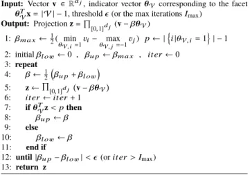
Algorithm 1 Bisection Method Iterative Check Polytope Projection Algorithm
Input: Vectorv ∈Rdj, indicator vectorθV corresponding to the facet θTVx=| V | −1, threshold(or the max iterationsImax)
Output: Projectionz=Q
[0,1]d j (v−βθV) 1: βm a x←12(θmin
V,i=1vi−θmax
V,j=−1vj) p← |(
i|θV,i=1)
| −1 2: initialβl ow←0 , βu p←βm a x , iter←0
3: repeat 4: β←12
βu p+βl ow 5: z←Q
[0,1]d j v−βθV 6: iter←iter+1 7: ifθTVz<pthen 8: βu p←β 9: else 10: βl ow←β 11: end if
12: until|βu p−βl ow|< (oriter>Imax) 13: return z
ing (BPSK) modulation. In the simulation experiment, the ADMM-LP decoder with penalty function l2 [10] is em- ployed. Based on[10], we can obtain a set of parameters (include the penalty parameterµand the parameterα) for a particular code that achieves the lowest FER by exhaustive search over all possible parameters. In this paper, we mainly consider the influence of different check polytope projec- tion algorithms on the performance of ADMM-LP decoder.
Therefore, we select a same set parameters that achieves low FER for simulation codes. The penalty parameterµis set to 2.2 and the parameterαis set to 3.0. Besides, the maximum number of iterations in ADMM decoding algorithm is set to 300.To illustrate the performance of BMIA in ADMM-LP decoder, we use the irregular (576, 288) rate 1/2 codeC1and (576, 192) rate 2/3 codeC2as well as regular (576, 96) rate 5/6C3from IEEE 802.16e. The check degree ofC1,C2and C3 are {6,7}, {10,11} and 20, respectively. In simulation, the frame error rate (FER) curve of the decoder with CSA is used as reference curve to determine whether the FER performance of decoder with BMIA (or Iterative check poly- tope projection algorithm) is optimal. If the decoder with BMIA (or Iterative check polytope projection algorithm) has a performance practically identical to that of CSA, the FER performance of decoder with BMIA (or Iterative check poly- tope projection algorithm) is optimal.
Figure 1 shows the effects of Imax and on the FER curves of the BMIA, demonstrating that both the Imaxand will affect the performance of the FER curve. We note that the FER curve tends to that of CSA gradually with the increasing of Imax ( = 0) (or with the decreasing of (Imax =∞)), especially when theis 0.01, the FER perfor- mance is optimal. Afterwards, we focus on comparing the performance of BMIA with the existing iterative projection algorithm (mainly the algorithm referred in[6]).
Table 1 shows the comparison of the average projection time of 30 iterations between BMIA and Iterative projection algorithm at signal-to-noise rate (SNR)=2.6, 3.2, 4.2 dB for
Fig. 1 FER performance ofC1for ADMM decoder with BMIA projec- tion algorithm for differentandIm a x.
Table 1 Avg. projection time.
Codeword Parity Check Polytope Projection Algorithm
Iterative BMIA
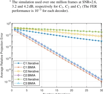
C1 8.8207×10⁻⁷ 8.6076×10⁻⁷ C2 1.1951×10⁻⁶ 1.0907×10⁻⁶ C3 2.07×10⁻⁶ 2.0489×10⁻⁶ 1The simulation used over one million frames at SNR=2.6,
3.2 and 4.2 dB, respectively forC1,C2andC3(The FER performance is 10−3for each decoder).
Fig. 2 Relative projection error ofC1,C2andC3for ADMM decoder with BMIA and Iterative projection algorithm for different iterations.
C1,C2 andC3, respectively. As shown in table, there is al- most no difference in the projection time between BMIA and Iterative algorithm under the same conditions (Imax =100, = 0, SNR= 2.6, 3.2, 4.2 dB forC1,C2 andC3, respec- tively). The result demonstrates that, for each iteration, the computational complexities of BMIA and Iterative algorithm are almost equal.
Figure 2 describes the relationship between the number of iterations and the average relative projection error. The relative error is calculated as | |z−z| |zt r u et r u e| || |22 (ztr ue denotes the accurate projection) at each projection. For each simulation point, 35000 frames are obtained. As shown in Fig. 2, for
Fig. 3 FER performance ofC1,C2andC3for ADMM decoder with BMIA and Iterative projection algorithm for differentIm a x.
BMIA and Iterative projection algorithm, the average rela- tive projection errors between the output projection and the accurate projection are decreasing as the number of iteration increase. It is intuitive that the speed of BMIA relative error decreasing is much faster than that of Iterative algorithm.
Especially after the iteration number reaches 10 iterations, the average relative error of BMIA is closer to zero.
Figure 3 shows the relationship between the FER perfor- mance of the decoders with BMIA and Iterative projection algorithm for different codewords. According to the FER curves ofC1,C2andC3, it’s obvious that with the increase of Imax, the FER curves of BMIA and Iterative algorithm approach to the CSA FER curve gradually. However, the approaching rate of BMIA and Iterative algorithm are not the same. Especially when the dimension is 20, the FER performance of BMIA has a practically identical to that of CSA after 8 iterations, but FER curve of Iterative algorithm takes 100 iterations to approach the performance of CSA.
Finally, it is worth noting that when the average relative projection errors for BMIA is a little more than that of Iter- ative projection algorithm, the FER performance for BMIA is intuitively better than that of Iterative algorithm. For ex- ample, when the iteration of BMIA is 4 and the iteration of Iterative projection algorithm is 20, the average relative pro- jection errors of BMIA is more than that of Iterative projec- tion algorithm, while the FER performance ofC1for BMIA is better than that for Iteartive projection algorithm. The projection ofv ontoPdj are given byQ
[0,1]d j (v−s∗θV), Q
[0,1]d j (v−βB M I AθV), Q
[0,1]d j (v−βI terθV) for cor- rect projection, BMIA and Iterative projection algorithm, respectively. Based on the algorithm of BMIA and Iterative projection algorithm respectively, the value of βB M I Acould be greater than, less than or equal tos∗, while the value of βI teris always less thans∗[6]. Therefore, when the average relative projection errors for BMIA and Iterative projection algorithm are identical, the estimate projection calculated by BMIA might lie inside the check polytope, while that of Iterative projection algorithm must be outside of check poly- tope. To further verification, under the same average relative
Fig. 4 FER performance ofC1for ADMM decoder with differentβat 3.4 dB
projection errors, the simulation explores the FER perfor- mances of codeC1at 3.4 dB for the case of β=s∗±δand β=s∗−δ(δ >0), respectively. As shown in Fig. 4, under the same average relative projection errors, the FER perfor- mance of decoder satisfying the projection possibly within the check polytope is better than that of decoder satisfying projection being outside of the check polytope.
5. Conclusion
To conclude, we propose a bisection method iterative algo- rithm in this paper. Compared with the existing projection algorithms, it does not require any sort operation, and the complexity of the algorithm is linear. Additionally, in com- parison with the existing iterative projection algorithm, the proposed projection algorithm reduces the number of itera- tions without affecting the decoding performance. When the dimension of input vector is high, the number of iterations for the performance of the decoder with BMIA reaching optimal
is only 1/10 of the iterative projection algorithm.
Acknowledgments
This work was supported by the National Natural Science Foundation of China (61501334), The Fundamental Re- search Funds for the Central Universities (CCNU16A05028).
References
[1] S. Barman, X. Liu, S.C. Draper, and B. Recht, “Decomposition methods for large scale LP decoding,” IEEE Trans. Inf. Theory, vol.59, no.12, pp.7870–7886, Dec. 2013.
[2] H. Wei, X. Jiao, and J. Mu, “Reduced-complexity linear program- ming decoding based on ADMM for LDPC codes,” IEEE Commun.
Lett., vol.19, no.6, pp.909–912, June 2015.
[3] X. Jiao, J. Mu, Y.C. He, and C. Chen, “Efficient ADMM decoding of LDPC codes using lookup tables,” IEEE Trans. Commun., vol.65, no.4, pp.1425–1437, Jan. 2017.
[4] X. Zhang and P.H. Siegel, “Efficient iterative LP decoding of LDPC codes with alternating direction method of multipliers,” Proc. IEEE Int. Symp. Inf. Theory, pp.1501–1505, Istanbul, Turkey, July 2013.
[5] G. Zhang, R. Heusdens, and W.B. Kleijn, “Large scale LP decoding with low complexity,” IEEE Commun. Lett., vol.17, no.11, pp.2152–
2155, Nov. 2013.
[6] H. Wei and A.H. Banihashemi, “An iterative check polytope pro- jection algorithm for ADMM-based LP decoding of LDPC codes,”
IEEE Commun. Lett., vol.22, no.1, pp.29–32, Jan. 2018.
[7] I. Debbabi, N. Khouja, F. Tlili, B.L. Gal, and C. Jego, “Multicore im- plementation of LDPC decoders based on ADMM algorithm,” IEEE International Conference on Acoustics, Speech and Signal Process- ing, pp.971–975, Shanghai, China, March 2016.
[8] X. Liu, ADMM Decoding of LDPC and Multipermutation Codes:
From Geometries to Algorithms, Ph.D. thesis, University of Wiscon- sin, Madison, USA, 2015.
[9] X. Zhang, LDPC Codes–Structural Analysis and Decoding Tech- niques, Ph.D. thesis, University of California, San Diego, USA, 2012.
[10] X. Jiao, H. Wei, J. Mu, and C. Chen, “Improved ADMM penalized decoder for irregular low-density parity-check codes,” IEEE Com- mun. Lett., vol.19, no.6, pp.913–916, June 2015.