The middle-income trap from the viewpoint of
trade structures
著者
Kumagai Satoru
権利
Copyrights 日本貿易振興機構(ジェトロ)アジア
経済研究所 / Institute of Developing
Economies, Japan External Trade Organization
(IDE-JETRO) http://www.ide.go.jp
journal or
publication title
IDE Discussion Paper
volume
482
year
2014-11-01
INSTITUTE OF DEVELOPING ECONOMIES
IDE Discussion Papers are preliminary materials circulated to stimulate discussions and critical comments
Keywords: middle-income trap, Malaysia, trade structure, flying geese JEL classification: O10,F14, O53
* Visiting Fellow, Malaysian Institute of Economic Research, Research Fellow Sent
IDE DISCUSSION PAPER No. 482
The Middle-income Trap from the
Viewpoint of Trade Structures
Satoru KUMAGAI*
November 2014
Abstract
In this study, we try to elucidate the middle-income trap from the viewpoint of international trade. We conduct regression analyses on the relationship between income level and net export ratios for different types of goods for trapped and non-trapped samples separately. Our findings indicate that industrial upgrading appears to occur exactly as depicted by the flying-geese model for non-trapped countries while trapped countries tend to depend on the export of primary commodities, and industrialization appears to be driven by forward linkages to processed goods and a narrow base. The results of our analyses suggest that the middle-income trap is a form of Dutch disease or a ‘resource curse’ in the middle-income stage.
The Institute of Developing Economies (IDE) is a semigovernmental, nonpartisan, nonprofit research institute, founded in 1958. The Institute merged with the Japan External Trade Organization (JETRO) on July 1, 1998. The Institute conducts basic and comprehensive studies on economic and related affairs in all developing countries and regions, including Asia, the Middle East, Africa, Latin America, Oceania, and Eastern Europe.
The views expressed in this publication are those of the author(s). Publication does not imply endorsement by the Institute of Developing Economies of any of the views expressed within.
INSTITUTE OF DEVELOPING ECONOMIES (IDE), JETRO 3-2-2, WAKABA,MIHAMA-KU,CHIBA-SHI
CHIBA 261-8545, JAPAN
©2014 by Institute of Developing Economies, JETRO
No part of this publication may be reproduced without the prior permission of the IDE-JETRO.
The Middle-income Trap from the Viewpoint of Trade Structures
Satoru KUMAGAI MIER/IDE-JETRO Abstract
In this study, we try to elucidate the middle-income trap from the viewpoint of international trade. We conduct regression analyses on the relationship between income level and net export ratios for different types of goods for trapped and non-trapped samples separately. Our findings indicate that industrial upgrading appears to occur exactly as depicted by the flying-geese model for non-trapped countries while trapped countries tend to depend on the export of primary commodities, and industrialization appears to be driven by forward linkages to processed goods and a narrow base. The results of our analyses suggest that the middle-income trap is a form of Dutch disease or a ‘resource curse’ in the middle-income stage.
Keywords: middle-income trap, trade structure, flying geese, Malaysia JEL classification: O10, F14, O53
Introduction
The middle-income trap (MIT) is a concept that has become popular among development agencies (ADB, 2012) and policy makers, including the Malaysian government. The MIT is a situation in which middle-income countries are not competitive with low-income countries in industries that utilize abundant low-wage workers, and are not competitive with high-income countries in industries that are research and development (R&D) intensive. It is believed that a country cannot become fully developed without avoiding or escaping this trap.
However, the theoretical foundation of this argument is surprisingly weak, with only a few papers exploring the foundation. Typically, Latin American countries are used as
examples of countries in the MIT. This raises the question: Is the MIT just a fear of lowering economic growth in the future, as in the case of East Asia?
This study seeks to understand what the MIT is and to identify possible mechanisms that would cause a country to fall into it, analyzing this from the viewpoint of international trade. Specifically, we investigate the relationship between income level and net export ratio (NXR) for different types of goods and formulate the MIT as a situation within which major industries have peaked and promising next-stage industries have not developed. This ‘flying-geese’ view of the MIT enables policy makers to formulate recommendations that actually help an affected country to climb the ladder and become a fully developed economy.
This paper is structured as follows. The literature related to the MIT is identified and briefly summarized in Section 1. In Section 2 we define MIT and use this definition to identify trapped countries and the relevant time periods. In Section 3 we report the results of regression analyses on the relationship between income level and NXRs for different types of goods in order to reveal differences in trade structures between trapped and non-trapped countries. In Section 4 we conclude the paper, with special reference to Malaysia.
1. Literature overview
There are a number of relevant studies on the MIT that have been published since 2007 when Gill et al. (2007) highlighted the concept of the MIT in An East Asian Renaissance. They showed that, for middle-income countries, it becomes more difficult to maintain historical growth rates by only factor accumulation due to a decline in the marginal productivity of capital. The authors argue that the key to escaping the trap is by exploiting economies of scale. Their argument is very clear and in the same vein as that in Krugman (1994). The argument is based on the economic concept of convergence, which is a consequence of the standard growth model. Within this, the growth rate of per capita income for a country becomes lower and tends toward zero as it approaches the steady state, assuming there is no technology growth in the economy.
Eechhout and Jovanovic (2007) provide another argument for the MIT, approaching the topic from the viewpoint of international economics. They construct an economic model with waged work and managerial work, within which people can choose between these two alternatives. In this setting, rich and poor countries gain more when economies are integrated, while middle-income countries gain less because they experience the smallest changes in the factor–price ratio. This argument is quite straightforward from the viewpoint of standard international economics. A possible factor, which is overlooked in the paper, is that semi-skilled workers, such as middle-tech engineers and experienced production managers are abundant in middle-income countries relative to that in richer and poorer countries makes these middle-income countries also gain from economic integration.
The micro aspects of the MIT are also put forward as contributory factors, mainly by Ohno (2009, 2010). The author uses the analogy of a glass ceiling to explain the MIT. The author categorizes industrial upgrading driven by foreign direct investment (FDI) into stages, from stage zero to four, and suggests that there is a glass ceiling for the Association of Southeast Asian Nations (ASEAN) countries between stage three, in which a number of local small and medium enterprises (SMEs) appear but still need foreign guidance, and stage four, in which local firms have mastered management and technology and can successfully produce high quality goods.
The hypothesis put forward by Jankowska et al. (2012) is a combination of the above two perspectives. The authors applied product-space analysis, in the manner of Hausmann et al. (2007), to East Asian and Latin American countries and found that successful Asian economies first diversified their export goods and then upgraded by concentrating on higher quality industries. They argue that the policies which facilitate the structural transformation process are essential to escaping from the MIT.
In a study by the Asian Development Bank (ADB, 2011), the MIT is seen as a risk for Asia and is contrasted with the “Asian Century” scenario, in which Asia’s share of world GDP becomes 51% by 2050. The ADB warned that in the MIT scenario the total
GDP of Asia would remain at only 41% of the more optimistic estimate. Around the time of this study, MIT became a major concern for governments, international organizations, media, and research institutes.
In some of the literature, attempts are made to identify which countries are actually trapped in the middle-income stage. Felipe (2012) defines the MIT as less than average speed while passing through the middle-income category. From 1950–2010 data about 124 countries, the author determined the average time taken to graduate from the lower-middle income category as being 28 years, and 14 years to graduate from the higher-middle income category. According to these guidelines, the Asian countries are currently trapped are Malaysia, Sri Lanka, and the Philippines.
Aiyar et al. (2013) adopted a different approach. They define the MIT as sudden and sustained deviations from the ordinary growth path predicted by a standard conditional convergence framework. They analyzed data to identify trapped countries and the relevant time periods. In the case of Malaysia, the author identified two trapped periods: 1980–1985 and 1995–2000.
Among the literature that focuses mainly on Malaysia, Yusuf and Nabeshima (2009) is the first study of the MIT and is the most comprehensive. Flaaen et al. (2013) briefly analyze Malaysia’s export structure for both goods and services and conclude that the key to avoiding the MIT in Malaysia is to modernize the service sector.
2. Identifying cases of the middle-income trap
2.1 Definition of middle-income
The MIT is different from the poverty trap at the lower level of income stage and from the normal convergence of the growth rate at a higher level of income stage. The MIT for a country is therefore caused, by definition, by being in a middle-income stage.
Thus, we first need to define the criteria for the category of middle-income. The World Bank publishes a widely used criterion for middle-income every year in its World Development Report. For the year 2013, middle-income was defined as a per capita income between USD 1,029 and 12,170, using nominal exchange rates calculated by the Atlas method. In addition to this, the income stage is divided into lower middle-income and upper middle-middle-income, at a threshold of USD 4,086.
Here, we define middle-income as GDP per capita between 1.95% and 23.75% of that of the USA in the same year. This is based on the World Bank criteria of middle income, mentioned above, normalized by the per-capita GDP of the USA. The threshold of 7.69% divides lower middle-income and upper middle-income.
2.2 Definition of trap
Although there is no single definition of the trap, it is taken to mean that something has gone awry in an economy and that it will last for some length of time. This is often express as economic stagnation, but the definition of stagnation is itself ambiguous. There are also issues in defining the length of stagnation that would categorize the situation as a trap rather than as an ordinary economic slowdown.
Here, we use the real growth rate of GDP per capita in local currencies1 as the indicator of economic growth. When the growth rate is zero or negative for at least a decade, then we classify that period as trapped. For example, if the average growth rate of GDP per capita for a country between 1965 and 1975 is less than zero, then we mark 1965 as the starting year of a trapped period. In contrast, if the average growth rate for the same country between 1966 and 1976 is above zero, we mark 1966 as being non-trapped, although it falls under the trapped period that started in 1965.
2.3 Identifying trapped countries and trapped periods
1
It is more appropriate to use growth rates in local currencies than in USD because GDP in USD is largely affected by the exchange rate both in the short run and the long run.
We sought to separate trapped and non-trapped periods by using unbalanced panel data covering 198 countries during 1960–2000. Table 1 shows the number of trapped periods by income level. As can be observed, the incidence of trapped periods decreases as income level increases. Both lower-middle income countries (LMCs) and upper-middle income countries (UMCs) experienced a lower incidence of trapped periods than low-income countries (LICs) did. High-low-income countries (HICs) are revealed to have the lowest incidence of trapped periods. These observations appear to be consistent with poverty trap arguments.
Table 1: Number of trapped/non-trapped periods by income level (1960–2000)
Source: Calculated from World Development Indicators Database
Table 2 shows the number of trapped periods by decade. The 1960s refers to the decade 1960-1969 (inclusive), with other decades analogously defined. The table shows that the incidence of trapped periods was higher in the 1970s and 1980s, while incidences in the 1960s and the 1990s were markedly lower.
Table 2: Number of trapped/non-trapped periods by decade (1960–2000)
(Source) Calculated from World Development Indicators Database
Trapped Non-Trapped Total % of trapped cases
LICs 317 745 1062 29.8%
LMCs 502 1372 1874 26.8%
UMCs 180 1048 1228 14.7%
HICs 81 1583 1664 4.9%
Total 1080 4748 5828 18.5%
Trapped Non-Trapped Total % of trapped cases
1960s 140 1090 1230 11.4%
1970s 361 933 1294 27.9%
1980s 436 1181 1617 27.0%
1990s 143 1544 1687 8.5%
Table 3 shows the number of trapped periods by region. The region with the highest proportion of trapped periods was Africa (37%), followed by Easter Europe (29%), Middle-East (22%) and Latin America (14%). In Asia, China (1 period, 1960–1969), Philippines (10 periods, from 1975–1984 to 1984–1993) and Mongolia (9 periods, from 1982–1991 to 1990–1999) are included in the set of trapped periods.
Table 3: Number of trapped/non-trapped periods by region (1960–2000)
(Source) Calculated from World Development Indicators
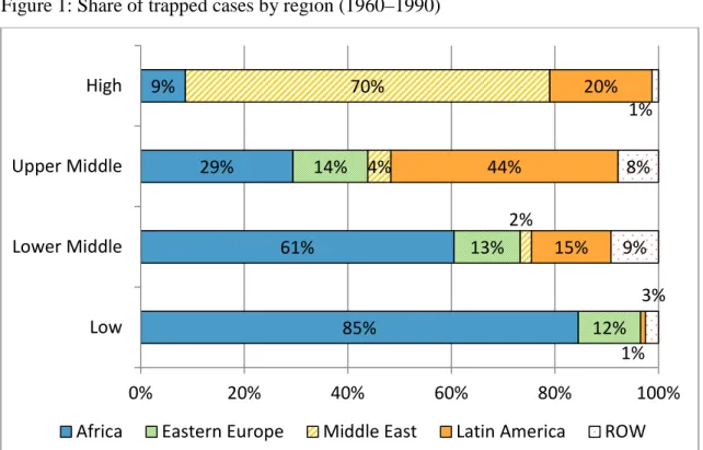
Figure 1 shows the proportion of each region that underwent trapped periods by income level. For the high-income countries, Middle Eastern countries account for 70% of all trapped periods. For the upper middle-income cases, Latin American countries account for 44% of all trapped periods. For the lower middle-income cases, African countries account for 61% of all trapped periods. For the low-income cases, African countries account for 85% of all trapped periods. Across all income levels, East Asian and Southeast Asian countries contribute negligible shares of trapped periods. Thus, the MIT is principally a problem for Latin American and African countries.
Trapped Non-trapped Total % of trapped cases
Africa 632 1078 1710 37.0% Eastern Europe 128 307 435 29.4% Middle East 76 261 337 22.6% Latin America 175 1108 1283 13.6% South Asia 29 233 262 11.1% Oceania 19 294 313 6.1% East Asia 10 188 198 5.1% Southeast Asia 10 261 271 3.7% Western Europe 1 857 858 0.1% North America 0 113 113 0.0% Total 1080 4748 5828 18.5%
Figure 1: Share of trapped cases by region (1960–1990)
(Source) Calculated from World Development Indicators
Some researchers may argue that the criterion for a trapped period used in this paper, a 10-year average growth in per-capita GDP below zero percent, is too restrictive. Table 4 shows the incidence of trapped periods by income level as found by four different criteria for being trapped: 10-years at 0% (or less), 10 years at 2%, 5 years at 0%, and 5 years at 2%. As the data show, the incidence of trapped periods becomes unreasonably high when using the other three criteria. It is difficult to call the condition a trap if the trapped periods constitute more than half of all periods.
The analysis so far indicates that it is inappropriate to aggregate Latin American and African countries with East Asian and Southeast Asian countries when talking about the MIT. The traps that countries in the former two regions have experienced are very deep, and traps of this severity have been very infrequent for countries in the latter two regions.
Of particular note for this study, Malaysia has experienced no trapped periods according to our criterion. If we apply a broader criterion, however (in which 5-year average
85% 61% 29% 9% 12% 13% 14% 2% 4% 70% 1% 15% 44% 20% 3% 9% 8% 1% 0% 20% 40% 60% 80% 100% Low Lower Middle Upper Middle High
growth in per-capita GDP is less than 2%), then Malaysia was trapped from 1981–1985 to 1987–1991 and from 1996–2000 to 2000–2004. The former periods include the recession caused by declining prices of primary commodities, and the latter includes the recession caused by the Asian currency and financial crisis. However, if we adopt this criterion, most of the other Eastern Asian countries, including Singapore and Japan, exhibit some trapped periods. Thus, a criterion of five years at less than 2% growth seems inappropriate.
Table 4: Percentage of trapped periods under various criteria (1960–2000)
(Source) Calculated from World Development Indicators
3. Why do countries become trapped?
3.1 Net export ratio as an indicator of economic upgrading
There are various possible causes of the MIT. It appears, for example, to be associated with mismanagement of the macro economy, such as in cases of hyperinflation and extreme volatility in foreign exchange rates. Being trapped is also related to fluctuations in oil prices for some oil-exporting countries. Some countries affected by MIT have also suffered more severe social instability, including wars, civil wars, revolutions, and natural disasters.
Here, we analyze the causes of the MIT from the perspective of competitiveness in international trade. We analyze historical changes in export structures to determine whether countries’ industrial upgrading of export goods follows a smooth transition. We use the NXR for four types of goods, which differ in their degree of sophistication. The
10 years ≤ 0% 10 years ≤ 2% 5 years ≤ 0% 5 years ≤ 2%
LICs 29.8% 88.8% 66.3% 88.7%
LMCs 26.8% 81.7% 57.4% 83.0%
HMCs 14.7% 63.6% 38.8% 66.6%
HICs 4.9% 63.5% 24.1% 66.9%
four types of goods are capital goods with parts and components (CAP)2—consumption goods (CON), primary commodities (PRM), and processed goods (PCS). Each type of goods is defined by aggregating items of the Broad Economic Categories (BEC) classification3.
Figures 2 to 5 show the NXR of four types of goods within four countries. Korea and Malaysia provide examples of non-trapped countries while Algeria and Argentina provide examples of countries with trapped periods. In the case of Korea (Figure 2), the NXR of CON has always been positive, and it peaked by the end of the 1980s. In place of CON, the NXRs of CAP and PCS have been positive and increasing since the end of the 1990s. The NXR of PRM has always been negative because Korea is not rich in natural resources. It can be seen that the upgrading of export structure, from CON to CAP and PCS, has been going on since the end of the 1980s.
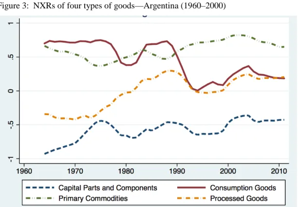
In contrast, Figure 3 shows that Argentina’s NXR of CON was large and positive until the end of the 1980s, but plunged to a neutral and then moderately positive value after that. The NXR of PCS improved to be positive from the beginning of the 1980s, but improvements in the NXR of CAP were modest and variable up to 2010. Argentina seems to be graduating from a net exporter of consumption goods, in a similar way to Korea, but the upgrading to capital goods and parts and components is slow. Argentina continues to be strongly competitive in the export of primary commodities.
2
We treated capital goods and parts and components separately at the beginning but found that these two goods show very similar characteristics in our analysis. So we aggregated these two goods for simplicity.
3
The classifications of goods are as follows: CAP (BEC 41,42, 521,53), CON (BEC 112,122,51,522,61,62,63), PRM (BEC 111,21,31), PCS (BEC 121,22,32).
Figure 2: NXRs of four types of goods—Korea (1960–2000)
(Source) COMTRADE database
Figure 3: NXRs of four types of goods—Argentina (1960–2000)
In the case of Malaysia, as shown in Figure 4, the NXR of PRM was positive in the 1970s but peaked by the end of 1980s, while the NXR of PCS remained between positive and neutral. The NXR of CON has been increasing and became positive by the end of the 1980s, and the NXR of CAP has increased to neutral since the beginning of the 2000s. It should be noted that Malaysia industrialized its export structure in the 1980s, and the industrial upgrading from CON to CAP has been going on gradually in that country.
Figure 4: NXRs of four types of goods—Malaysia (1960–2000)
(Source) COMTRADE database
Figure 5 shows the data for Algeria. As can be seen, the NXR of PRM remained very high while the NXR of CON decreased to almost –1 by the middle of the 1980s. The industrial upgrading to PCS had been progressing during the 1980s and the 1990s, but reverted to previous levels in the 2000s. The NXR of CON has remained negative and close to –1, indicating that Algeria shows no signs of transitioning to a net exporter of consumption goods. In comparison with Malaysia, Algeria seems to be failing to transform itself from a net exporter of primary commodities to a net exporter of manufacturing goods.
Figure 5: NXRs of 4 types of goods—Argentina (1960–2000)
(Source) COMTRADE database
3.2 Regression analysis
In this section, we explore the general patterns of changing NXRs for the four types of goods examined as a country’s income level increases. To achieve this, we calculated the estimated NXRs of the four types of goods against income level by quadratic regression. First, we constructed a dataset of NXRs for the four types of goods for each country during the period 1970–2005 at five-year intervals4. The NXRs are calculated as five-year averages, and the maximum time dimension for a country is eight. Following this, we combined our data with the per-capita GDP of each country in nominal USD, normalized by that of the USA in the same year. Finally, we separated the samples into trapped and non-trapped subsets according to the previously given criterion. To illustrate our approach we take the NXRs and per-capita GDP data for one country in 1970 as an example. If the country has at least one trapped year between
4
1970 and 1974 then the data are classified as trapped in our sample. If the country has no trapped year between 1970 and 1974, then the data are classified as non-trapped.
We regress the NXRs on log GDP per capita (GDPPC) and the square of log GDPPC for two separated samples as follows.
𝑁𝑋𝑅𝑖𝑡𝑘 = 𝛼𝑘+ 𝛽1𝑘𝑙𝑜𝑔(𝐺𝐷𝑃𝑃𝐶𝑖𝑡) + 𝛽2𝑘𝑙𝑜𝑔(𝐺𝐷𝑃𝑃𝐶𝑖𝑡)2+ 𝜀𝑖𝑡𝑘 …(1)
where 𝑁𝑋𝑅𝑖𝑡𝑘 is the NXR of goods k for country i in year t. 𝐺𝐷𝑃𝑃𝐶𝑖𝑡 is the USA-normalized GDP per capita for country i in year t.
The resulting estimates are shown in Table 5. Because the logarithm is applied to the USA-normalized GDPPC, the intercept is the estimated NXR value at the GDPPC of the USA.
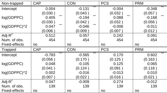
Table 5: Regression results for non-trapped and trapped samples
Non-trapped CAP CON PCS PRM
Intercept 0.004 -0.131 *** -0.004 -0.348 *** (0.030 ) (0.043 ) (0.032 ) (0.057 ) log(GDPPC) 0.405 *** -0.194 *** 0.088 *** -0.168 *** (0.030 ) (0.042 ) (0.032 ) (0.056 ) log(GDPPC)^2 0.047 *** -0.046 *** -0.006 -0.011 (0.006 ) (0.009 ) (0.007 ) (0.012 ) Adj-R2 0.512 0.057 0.242 0.091 Num. of obs. 454 454 454 454 Fixed-effects no no no no
Trapped CAP CON PCS PRM
Intercept -0.783 *** -0.565 *** 0.170 0.602 *** (0.056 ) (0.170 ) (0.125 ) (0.163 ) log(GDPPC) 0.048 -0.105 0.125 0.065 (0.041 ) (0.124 ) (0.091 ) (0.118 ) log(GDPPC)^2 0.002 -0.016 -0.013 0.010 (0.007 ) (0.022 ) (0.016 ) (0.021 ) Adj-R2 0.047 -0.009 0.274 -0.012 Num. of obs. 139 139 139 139 Fixed-effects no no no no
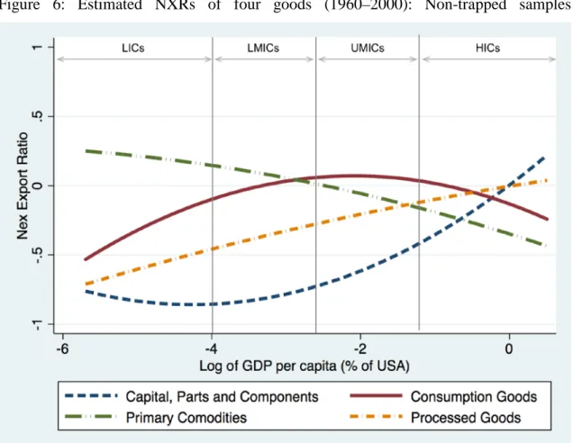
For non-trapped samples (Figure 6), the estimated NXRs of PRM are positive for low and lower-middle income levels but become negative as income level increases. The estimated NXR of CON increases as income level increases, but peaks at the upper-middle income stage. The NXRs for PCS and CAP are shown to be increasing as
income level increases. This produces precisely the flying-geese diagram for a country with a multi-goods model (see Appendix). As the income level of a country increases it tends to export more sophisticated goods.
Figure 6: Estimated NXRs of four goods (1960–2000): Non-trapped samples
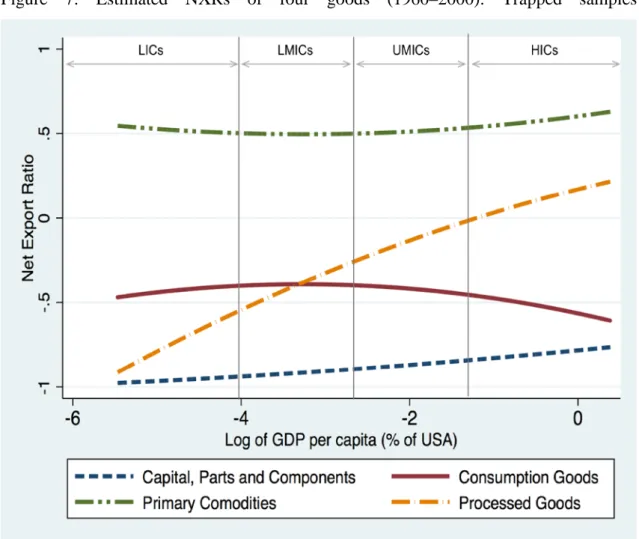
In contrast the results for the trapped samples (Figure 7) are significantly different from those of the non-trapped samples because the NXR of PRM is always positive, regardless of income level. The NXRs of CON and CAP are negative, regardless of income level. Only the NXR of PCS increases as income level increases, which agrees with the behavior of non-trapped samples.
Figure 7: Estimated NXRs of four goods (1960–2000): Trapped samples
Table 6 shows the correlations between the NXRs of two types of goods by income level. As can be seen, CAP, CON, and PCS have positive correlations with each other, regardless of income levels. It is also notable that the positive relationship between CAP and CON is the strongest. Because CAP is more sophisticated than CON, and the correlation coefficient is increasing with income level, it seems that industrial upgrading through the backward linkage from CON to CAP is a likely path.
In contrast, the relationships between PRM and CON and between PRM and CAP are both negative. This indicates that it is difficult for a country to be a net exporter of either both PRM and CON or both PRM and CAP. Thus, the net exporters of primary commodities are less likely to experience increased industrialization though a backward linkage from CON to CAP.
Table 6: Correlation between NXRs of two product types by income level
LICs LMCs UMCs HICs All
CAP-CON 0.35 0.43 0.53 0.56 0.47 CAP-PCS 0.45 0.35 0.27 0.41 0.37 CON-PCS 0.26 0.20 0.17 0.28 0.23 PRM-PCS -0.20 -0.12 0.10 0.01 -0.05 PRM-CAP -0.13 -0.44 -0.19 -0.56 -0.33 PRM-CON -0.51 -0.36 -0.24 -0.46 -0.39
It is possible to characterize differences in industrial upgrading path for trapped countries and non-trapped countries as follows. For non-trapped countries, the export structure shifts from primary commodities to consumption goods, then processed goods to capital goods, parts and components, as postulated in the flying-geese model of Akamatsu (1962). In that model, the driving force of industrial upgrading is the backward linkages from consumption goods to capital goods and parts and components.
Trapped countries, in contrast, rely on exports of primary commodities regardless of income level, and the competitiveness of consumption goods remains low relative to that of non-trapped samples in the same income categories. The NXR of capital goods and parts and components is not found to increase even at the high-income level. Trapped countries appear to fail to develop manufacturing industries other than within the processed goods sector and it is therefore understandable that the economic development achieved through this route leads to the MIT, because industrialization is likely to remain narrowly based.
3.3 Refined regression analysis using fixed effects models
In this section we conduct more statistically robust analyses of the relationship between the NXRs of four types of goods and income level. To make the estimate unbiased, we need to use fixed-effect estimator. We cannot estimate all country characteristics for
this, but we can control some for characteristics that are stable in the long term, such as natural resource endowment, geographical location, language, history, and cultural aspects as well as the fundamental characteristics of the law and national institutions.
We conducted fixed-effects regressions according to the following equation; the results are shown in Table 7.
𝑁𝑋𝑅𝑖𝑡𝑘 = 𝛼𝑘+ 𝛽1𝑘𝑙𝑜𝑔(𝐺𝐷𝑃𝑃𝐶𝑖𝑡) + 𝛽2𝑘𝑙𝑜𝑔(𝐺𝐷𝑃𝑃𝐶𝑖𝑡)2+ 𝜖𝑖𝑘+ 𝑢𝑖𝑡𝑘 … (2)
where the error term in equation (1) is divided into the unobserved time-invariant individual effect( 𝜖𝑖𝑘 ) and the error term(𝑢𝑖𝑡𝑘).
Table 7: Regression results for non-trapped and trapped samples
Non-trapped CAP CON PCS PRM
Intercept -0.412 *** -0.447 *** -0.234 -0.102 (0.067 ) (0.086 ) (0.066 ) (0.105 ) log(GDPPC) 0.094 * -0.241 *** 0.030 -0.056 (0.067 ) (0.065 ) (0.050 ) (0.079 ) log(GDPPC)^2 0.011 -0.017 0.008 -0.011 (0.010 ) (0.013 ) (0.010 ) (0.015 ) Adj-R2 0.012 0.065 0.002 0.002 num. of obs. 454 454 454 454
fixed-effects yes yes yes yes
Trapped CAP CON PCS PRM
Intercept -1.007 *** -1.109 *** -0.590 ** 0.656 *** (0.093 ) (0.191 ) (0.265 ) (0.239 ) log(GDPPC) -0.065 -0.343 *** -0.202 -0.017 (0.056 ) (0.116 ) (0.160 ) (0.021 ) log(GDPPC)^2 -0.008 -0.029 * -0.030 -0.021 (0.008 ) (0.017 ) (0.023 ) (0.145 ) Adj-R2 0.018 0.161 0.020 0.064 num. of obs. 139 139 139 139
fixed-effects yes yes yes yes
Figure 8 shows the relationship between NXRs and income level for non-trapped samples after controlling for country fixed effects. The figure shows that the NXR of CON decreases as the income level increases. In contrast, the NXRs of PRM and PCS are not affected by income level and the NXR of CAP increases slightly as income reaches the high-income stage.
Figure 8: Estimated NXRs of four goods, fixed-effect estimator (1960–2000): Non-trapped samples
Figure 9 shows the relationship between NXRs and income level for trapped samples after controlling for country fixed effects. As shown, the NXR of CON decreases as income level increases. In contrast, the NXR of PRM appears to be increasing as income level increases, although this is statistically insignificant (see Table 7). The NXRs of PCS and CAP are unaffected by the income level.
Figure 9: Estimated NXRs of four goods, fixed-effect estimator (1960–2000): Trapped samples
The fixed effects estimates do not change the hypothetical growth paths derived in the previous section. This is because, first, the trapped samples depend on the exports of primary commodities even at high-income levels. Second, the NXRs of consumption goods decrease as the income level increases for both samples, but the intercept for trapped samples is significantly lower than that for non-trapped samples. Third, the NXR of capital goods, parts, and components remains low for trapped samples. These results lead us to the same conclusion as those of the previous section: non-trapped countries successfully industrialize and upgrade to capital goods, parts, and component manufacturing, while trapped countries continue to export primary commodities and processed goods at a higher income level.
4. Conclusions
In this paper, we proposed a definition for the MIT and identified trapped countries and periods. According to the criterion for MIT used in this paper, most of the trapped periods occur in Africa or Latin America. For East Asia and Southeast Asia, there are only a very small number of trapped cases. Therefore, we argue that it is not appropriate to analyze the risk of the MIT for East Asian countries within the context of Latin American and African countries.
From the analyses of NXRs for four types of goods it was possible to derive plausible explanations to account for differences between trapped and non-trapped countries. For non-trapped countries, the industrial upgrading process appears to be consistent with the flying-geese model. It is therefore possible to conclude that the industrial upgrading process through the backward linkage from consumption goods to capital goods, parts, and components is more successful in non-trapped higher income countries. For trapped countries, there is a tendency to depend on the exports of primary commodities, and industrialization would appear to be driven by the forward linkage to processed goods. This narrow industrial base is thus a possible cause of the MIT. These analyses lead us to suspect that the MIT can be characterized as a form of Dutch disease or resource curse at the middle-income stage.
The policy implications from the findings of this paper are rather straightforward in many ways. They suggest that that it is necessary to develop the consumption goods industry and maintain competitiveness for as long as possible while facilitating industrial upgrading to capital goods, parts, and components by means of backward linkages. However, our findings clearly show that the development of the processed goods sector alone does not guarantee that a county can avoid the MIT.
For Malaysia, an extreme sluggishness in the economy such as zero growth over a decade is unlikely because of its export structure. However, in the past Malaysia has experienced periods when it was on the verge of being a trapped country. The findings of this study show that in the early 1980s the NXR of PRM for Malaysia was high,
while for PCS it was positive. In contrast the NXRs of CON and CAP were both negative. This is a typical pattern of NXRs in countries experiencing trapped periods.
Fortunately for Malaysia, it had changed this NXR structure by the end of the 1980s; the NXR of CON was significantly improved and that of CAP followed. Today, Malaysia is one of those rare countries that exhibit strength in both manufacturing goods and primary commodities, and its export structure is very different from those of trapped samples. However, there are small signs of regressive steps toward the export structure of trapped samples. Recently, for example, the NXRs of PRM and PCS have been increasing, especially since 2000, partly because of an increase in the price of primary commodities. The NXR of CON, however, seems to have peaked, and the NXR of CAP is not increasing. If this trend continues, Malaysia is at risk of approaching the export structure of trapped samples.
APPENDIX: The flying-geese model of industrial upgrading
As first mentioned in Akamatsu (1935), the export structures of East Asian countries gradually shifted from goods with a lower level of sophistication to goods with higher sophistication. A country’s exports usually start with consumption goods, followed by parts and components and capital goods. The net exports of primary commodities tend to be turned into net imports as economic development progresses.
The basic pattern of the flying-geese model of economic development was proposed in Akamatsu (1935, 1937) and is described in the context of a one-country model. However, there are two versions of the country model: the country, one-product model and the one-country, multiple one-products model.
Flying geese: One-country, one-product model
The one-country, one-product model explains a historical pattern of the development of an industry in a country from the viewpoint of imports, exports, and the production of one specific product. Akamatsu explained this basic pattern as follows:
Wild geese fly in orderly ranks forming an inverse V, just as airplanes fly in formation. This flying pattern of wild geese is metaphorically applied to the below figured three time-series curves each denoting import, domestic production, and export of the manufactured goods in less-advanced countries (Akamatsu, 1962, p. 11).
The figure that Akamatsu describes above is consistent with that of Figure A1. Akamatsu (1962, p. 12) referred to this as the fundamental wild-geese-flying pattern.
Figure A1: Akamatsu’s fundamental flying-geese pattern of economic development
Akamatsu explained the fundamental pattern of the flying-geese model as belonging to the following four stages.
Stage 1: Import of manufactured consumer goods begins.
Stage 2: Domestic industry begins production of previously imported manufactured consumer goods while importing capital goods to manufacture those consumer goods.
Stage 3: Domestic industry begins exporting manufactured consumer goods.
Stage 4: The consumer goods industry catches up with similar industries in developed countries. Export of the consumer goods begins to decline, and the capital goods used for production of the consumer goods are exported.
Akamatsu’s fundamental model is based on the case of Japan’s industrial development before World War II, specifically industries involving cotton yarn and wool. He provides statistical evidence to support the flying-geese pattern in that context and provides a comprehensive picture of import, production, and export in Japan’s cotton yarn and wool industries from the 1860s to the 1930s (Akamatsu, 1935, 1937).
Flying geese: One-country, multiple products model
Akamatsu expanded the one-country, one-product model to the one-country, multiple products model in his first paper on the flying-geese model (Akamatsu, 1935). He compared the above one-country, one-product pattern of industrial development between the cotton yarn industry and the wool industry relative to final goods, intermediate goods, and capital goods within each industry. He found that there are sequential patterns in economic development both between and within industries.
Later, he generalized this pattern, indicating that “the time for the curves of domestic production and export to go beyond that of import will come earlier in crude goods and later in refined goods, and similarly, earlier in consumer goods and later in capital goods” (Akamatsu, 1962, p. 11).
Figure A2 is based on the above description. The vertical axis is the net export ratio of goods, used instead of the three lines of import, production, and export found in Figure 2. This represents the ‘flying-fish’ concept of industrial development; the inverse-V shape crosses the horizontal axis twice, metaphorically similar to a flying fish jumping from the surface of the sea before sinking below again.
Figure A2: Flying-fish diagram of industrial development for a Country
Mechanism behind the one-country, multiple products model
One of the problems associated with the flying-geese model relates to the fact that Akamatsu did not explain the mechanism behind the pattern with the terminology of neo-classical economics. He referred to his model as “a historical theory” (Akamatsu 1962, p. 11). Kojima (1960) offered the explanation that the accumulation of capital (the Heckscher–Ohlin factor) is the fundamental driving force of the flying-geese model. Kojima (2000) further mentioned the Ricardian advantage of learning-by-doing and economies of scale as driving forces. Later, Fujita and Mori (1999) tried to reproduce the multi-country, multiple products flying-geese pattern of economic development by using a simulation model of spatial economics (specifically, the new economic geography).
References
Akamatsu, K. (1935). Waga kuni yomo kogyohin no boueki susei. Shogyo Keizai Ronso 13: 129-212.
___________. (1937). Waga kuni keizai hatten no sougou bensyoho. Shogyo Keizai Ronso 15: 179-210.
___________. (1962). Historical pattern of economic growth in developing countries. The Developing Economies 1: 3-25.
Aiyar, M. S., Duval, M. R. A., Puy, M. D., Wu, M. Y., & Zhang, M. L. (2013). Growth slowdowns and the middle-income trap (No. 13-71). International Monetary Fund.
Yusuf, S., & Nabeshima, K. (2009). Tiger economies under threat: a comparative analysis of Malaysia's industrial prospects and policy options. World Bank Publications.
Eeckhout, J., & Jovanovic, B. (2007). Occupational sorting and Development. NBER working paper w13686.
Flaaen, A., Ghani, E., & Mishra, S. (2013). How to avoid middle income traps? evidence from Malaysia. Evidence from Malaysia (April 1, 2013). World Bank Policy Research Working Paper, (6427).
Jankowska, A., Nagengast, A., & Perea, J. R. (2012). The product space and the middle-income trap: Comparing Asian and Latin American experiences (No. 311). OECD Publishing.
Felipe, J. (2012). Tracking the Middle-Income Trap: What is It, Who is in It, and Why?: Part 1.
Gill, I. S., Kharas, H. J., & Bhattasali, D. (2007). An East Asian renaissance: ideas for economic growth. World Bank Publications.
Fujita, M., and Mori, T. (1999). A flying geese model of economic development and integration: Evolution of international economy a la East Asia (Vol. 493). Discussion Paper.
Hausmann, R., Hwang, J., & Rodrik, D. (2007). What you export matters. Journal of economic growth, 12(1), 1-25.
Kohli, H. S., Sharma, A., & Sood, A. (Eds.). (2011). Asia 2050: realizing the Asian century. SAGE Publications India.
Kojima, K. (1960). Capital accumulation and the course of industrialisation, with special reference to Japan. The Economic Journal LXX: 757-768
__________. (2000). “The “flying geese” model of Asian economic development: origin, theoretical extensions, and regional policy implications.” Journal of Asian Economics 11: 375-401.
Krugman, P. (1994). Myth of Asia's Miracle, The. Foreign Aff., 73, 62.
Ohno, K. (2009). Avoiding the middle-income trap: renovating industrial policy formulation in Vietnam. ASEAN Economic Bulletin, 26(1), 25-43.