Regional disparities in subjective well-being
: a spatial econometric approach
著者
Takeshi Aida
権利
Copyrights 2020 by author(s)
journal or
publication title
IDE Discussion Paper
volume
766
year
2020-03
INSTITUTE OF DEVELOPING ECONOMIES
IDE Discussion Papers are preliminary materials circulated to stimulate discussions and critical comments
Keywords: subjective well-being; spillover effect; regional disparities; spatial econometrics JEL classification: I31, R12, C31
* Research Fellow, Microeconomic Analysis Studies Group, Development Studies Center, IDE ([email protected])
IDE DISCUSSION PAPER No. 766
Regional Disparities in Subjective
Well-being: A Spatial Econometric
Approach
Takeshi AIDA*
March 2020
Abstract
This study aims to explore spatial externalities in subjective well-being (SWB) as sources of regional disparities. Although previous studies have shown positive externalities in SWB, the estimated effect is frequently confounded by unobserved regional heterogeneities, which can be sources of regional disparities. Using a household panel dataset collected in South Africa, the study estimates spatial econometric models with fixed effects to show spatial externalities in SWB by explicitly controlling for unobserved heterogeneities at the individual and regional levels. Estimation results indicate strong spatial dependence on SWB, confirming that spatial externalities within and across geographical clusters are essential factors for explaining regional disparities.
The Institute of Developing Economies (IDE) is a semigovernmental, nonpartisan, nonprofit research institute, founded in 1958. The Institute merged with the Japan External Trade Organization (JETRO) on July 1, 1998. The Institute conducts basic and comprehensive studies on economic and related affairs in all developing countries and regions, including Asia, the Middle East, Africa, Latin America, Oceania, and Eastern Europe.
The views expressed in this publication are those of the author(s). Publication does not imply endorsement by the Institute of Developing Economies of any of the views expressed within.
INSTITUTE OF DEVELOPING ECONOMIES (IDE), JETRO 3-2-2, WAKABA,MIHAMA-KU,CHIBA-SHI
CHIBA 261-8545, JAPAN
©2020 by author(s)
No part of this publication may be reproduced without the prior permission of the author(s).
Regional Disparities in Subjective Well-being: A Spatial Econometric Approach†
Takeshi Aida March 2020
Abstract
This study aims to explore spatial externalities in subjective well-being (SWB) as sources of regional disparities. Although previous studies have shown positive externalities in SWB, the estimated effect is frequently confounded by unobserved regional heterogeneities, which can be sources of regional disparities. Using a household panel dataset collected in South Africa, the study estimates spatial econometric models with fixed effects to show spatial externalities in SWB by explicitly controlling for unobserved heterogeneities at the individual and regional levels. Estimation results indicate strong spatial dependence on SWB, confirming that spatial externalities within and across geographical clusters are essential factors for explaining regional disparities.
Keywords: subjective well-being; spillover effect; regional disparities, spatial econometrics JEL classification: I31, R12, C31
Institute of Developing Economies, Japan External Trade Organization. Wakaba 3-2-2, Mihama-ku, Chiba-shi, Chiba 261-8545, Japan.
1. Introduction
After the pioneering work of Easterlin (1974), analysis of happiness or subjective well-being (SWB) data has become popular in social sciences in the last four decades. Its use is not limited to academia; hence, it is also becoming a popular index for policymakers (Stiglitz et al., 2009). The underlying presumption is that such subjective indices can measure the welfare of the people, albeit not perfectly. As supporting evidence, previous studies have shown several consistent patterns in the relationship between individual characteristics and SWB across region or countries (e.g., Dolan et al., 2008; Frey and Stutzer, 2002; MacKerron, 2012).
In addition to the consistent patterns in SWB, considerable differences in the level of SWB across region or countries are widely known (e.g., Pittau et al., 2010; Oswald and Wu, 2011; Aslam and Corrado 2012). Interestingly, such regional disparities remain even after controlling for individual characteristics. One method for explaining these disparities is attributing them to regional level heterogeneities in institutions and amenities. Indeed, previous studies have shown that political institutions and city environments are important determinants of SWB (e.g., Brereton et al., 2008; Frey and Stutzer, 2000; Hogan et al., 2016). Therefore, unobserved regional heterogeneities can be essential drivers of regional disparities in SWB.
Conversely, the literature in psychology arguing that SWB is “contagious” is growing, that is, people tend to feel happy when the surrounding people are happy (e.g., Fowler and Christakis, 2008; Ballas and Tranmer, 2012). Such spillover effect will also lead to regional disparities because people whose neighbors have high levels of SWB will also have high levels of SWB and vice versa. However, the estimated spillover effect is frequently confounded by regional heterogeneities, and identifying such spillover requires a rigorous econometric approach.
This study aims to test spatial externalities in SWB using the spatial econometric approach. Especially, the study focuses on whether externalities arise in SWB after controlling for heterogeneities at the individual and regional levels. For this purpose, micro-level panel data from South Africa are analyzed, where inequalities across municipalities are a very salient issue (e.g., Bosker and Krugell, 2008; Leibbrandt and Woolard, 1999). Two types of spatial externalities are investigated, namely, within and across-district municipalities. Within-district externality is analyzed using individual panel data to test whether people feel high levels of SWB when their neighbors have high levels of SWB. Conversely, across-district externality is analyzed using aggregated district-level panel data to test whether the average SWB is high in a district surrounded by districts with high average SWB.
Prior to the present study, several spatial econometric analyses on SWB have been carried out (Stanca, 2010; Lin et al., 2014; 2017). However, these studies use country or regional level data and overlook individual level spillover within a region. In addition, these studies exploit cross-sectional variations only, whereas unobserved heterogeneities at the regional level are not explicitly controlled. Another relevant study is Tumen and Zeydanli (2015), who show that no significant spillover in SWB was observed in the UK by estimating the multi-level linear-in-means model. The current study differs because the spillover effect is tested within and across geographical clusters by explicitly controlling for individual and regional level heterogeneities, which is difficult in multi-level analysis.
To preview the result, the study shows a significantly positive spatial spillover in SWB within a geographical cluster, which is robust to the inclusion of individual or regional level heterogeneities. To the best of the authors’ knowledge, this study is one of the first to find a significant micro-level spatial spillover in a developing country. Moreover, positive spillovers across clusters are confirmed after controlling for time-invariant heterogeneities, which supports the findings of previous studies analyzing cross-sectional data.
The remainder of the paper is structured as follows. Section 2 describes the data and discusses regional disparities in SWB in South Africa. Section 3 introduces the spatial econometric specification of SWB analysis. Section 4 discusses the estimation results. Lastly, Section 5 concludes.
2. Data
We analyze data collected by the National Income Dynamics Study (NIDS), which is the first nationally representative household panel data in South Africa. The project is implemented by the Southern Africa Labour and Development Research Unit (SALDRU) based at the University of Cape Town’s School of Economics. The unit has been conducting surveys every two years since 2008. Currently, a total of five rounds of survey data (i.e., 2008, 2010, 2012, 2014, and 2017) are available for analysis. The original sample size consisted of more than 28,000 individuals in 7,300 households. However, the study restricts the sample to each household head to lessen the computational burden, especially for the below-mentioned spatial econometric approach.
NIDS includes a wide variety of information, such as household demography, well-being, and human capital. In the dataset, SWB is probed by asking the following question: “Using a scale of 1 to 10 where 1 means ‘Very dissatisfied’ and 10 means ‘Very satisfied’, how do you feel about your life as a whole right now?” Figure 1 shows the histogram of SWB in
each round, which is distributed nearly symmetrically, although slightly right-skewed in rounds 2 and 3.
South Africa is an emerging economy whose GDP is one of the highest in the African continent. However, the country is also known to have the highest level of inequality worldwide, and high poverty incidence is an important social issue (e.g., Aida, 2018). Previous studies have documented the strong persistence of poverty (Finn and Leibbrandt, 2016; Agüero et al., 2007; Carter and May, 2001). In addition, racial differentials are a serious problem in the country, and a clear racial gap exists in poverty and deprivation due to the cumulative disadvantaged characteristics of Africans (Gardin, 2012).
A pattern of inequality can be found at the regional level, that is, income distribution is uneven across regions, which is diverging over time (e.g., Bosker and Krugell, 2008; Leibbrandt and Woolard, 1999). Furthermore, a strong spatial dependence and clustering are observed in poverty indices (David et al., 2018). These regional disparities in economic activity originate from the homeland policy during the Apartheid era, which had restricted the migration of the African people (Christopher, 1992). Although internal migration has increased after the Apartheid, migrants remain largely temporal (Posel, 2004).
Previous studies have explored not only the economic measures of welfare but also SWB in South Africa. In addition, several studies found that regional as well as individual level characteristics are essential determinants of SWB (e.g., Powdthavee, 2005; 2007; Kingdon and Knight, 2007). For this reason, together with income inequality across regions, regional disparities are expected to be salient in SWB as well.
As a measure of regional unit, the study focuses on the administrative division in South Africa. The country consists of nine provinces, each of which is governed by a unicameral legislature and a Premier elected by the legislature. The provinces are further divided into 52 districts (8 metropolitan municipalities and 44 district municipalities). These districts are used as the main unit of the regional cluster because they are the smallest administrative unit available in the dataset.
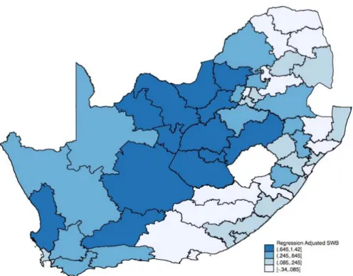
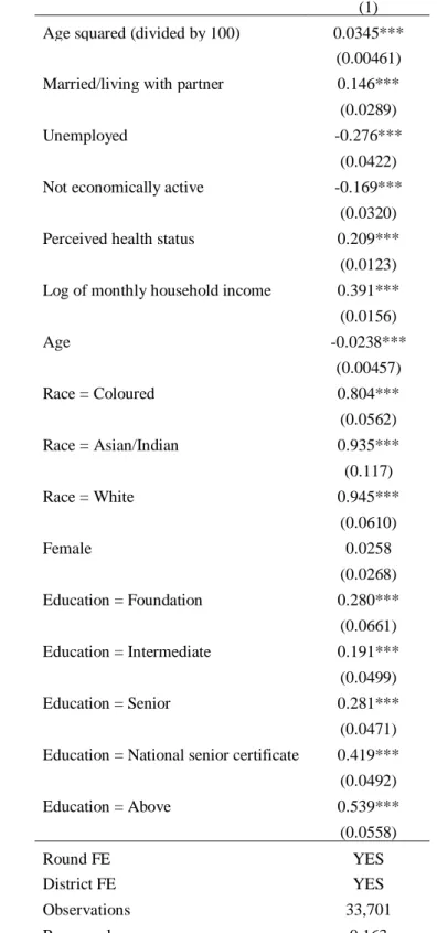
Before estimating the main spatial econometric models described below, testing whether regional disparities in SWB exist in the current dataset is crucial. Following Pittau et al. (2010) and Oswald and Wu (2011), the regression-adjusted SWB is calculated by estimating the OLS coefficient on district dummies after controlling for individual characteristics and round dummies.1 Appendix Table A1 provides the estimation results for other variables. The district dummies are jointly significant (F = 17.14), which confirms significant regional
disparities in SWB. Figure 2 presents a visualization of the coefficients of the district dummies using a heat map. The districts in the central part (e.g., Free State and North West Provinces) tend to exhibit high levels of SWB, whereas those in the Eastern Cape and Limpopo Provinces exhibit low levels of SWB. Furthermore, these casual observations imply spatial correlation in SWB across districts, which is in agreement with previous studies (e.g., Stanca, 2010; Lin et al., 2014; 2017)
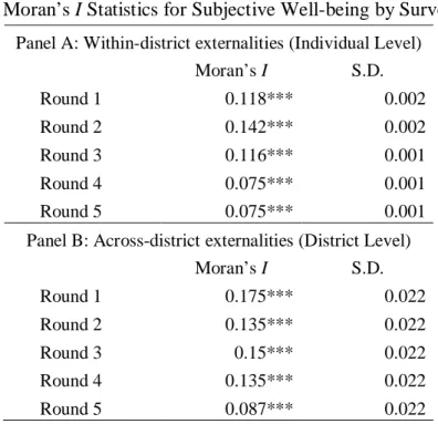
Testing whether a significant spatial correlation in SWB exists within and across districts is also informative. Panel A in Table 1 shows Moran’s I statistics by each survey round, using a weight matrix that takes a value of one if individuals i and j are in the same district. Otherwise, it takes a value of zero. Although the magnitudes of the coefficient are not necessarily very large, they are statistically significant. In addition to micro-level spillovers, the study tests for across-district spatial correlation with aggregated district-level data. Panel B shows district-level Moran’s I statistics using an inverse distance weight matrix. The coefficients are highly significant, and the magnitudes are comparable to micro-level within-district spatial correlation. Such results imply potential spatial spillovers in SWB within and across districts. However, our main interest is whether or not this significant spatial correlation remains even after controlling for individual and regional level heterogeneities. Toward this end, the study employs a spatial econometric approach.
3. Empirical Strategy
The study mainly aims to test whether the spatial externalities hold after controlling for individual and regional level heterogeneities. For this purpose, the study employs a spatial econometric approach, which has been developed to incorporate spatial dependence and heterogeneities (e.g., Anselin, 1988; LeSage and Pace, 2009). Specifically, the combined spatial lag and error (SAC) model with several types of fixed effects is estimated as follows:
𝑦𝑦𝑖𝑖𝑖𝑖 = 𝜌𝜌 � 𝑤𝑤𝑖𝑖𝑖𝑖𝑦𝑦𝑖𝑖𝑖𝑖 𝑁𝑁 𝑖𝑖=1 + 𝑥𝑥𝑖𝑖𝑖𝑖𝛽𝛽 + 𝛿𝛿𝑖𝑖 + 𝜁𝜁𝑖𝑖+ 𝑢𝑢𝑖𝑖𝑖𝑖 (1) 𝑢𝑢𝑖𝑖𝑖𝑖 = 𝜆𝜆 � 𝑤𝑤𝑖𝑖𝑖𝑖𝑢𝑢𝑖𝑖𝑖𝑖 𝑁𝑁 𝑖𝑖=1 + 𝜖𝜖𝑖𝑖𝑖𝑖,
where 𝑦𝑦𝑖𝑖𝑖𝑖 denotes the level of SWB, 𝑥𝑥𝑖𝑖𝑖𝑖 stands for the set of control variables, and 𝛿𝛿𝑖𝑖 and 𝜁𝜁𝑖𝑖 are individual and round fixed effects, respectively. 𝑤𝑤𝑖𝑖𝑖𝑖 pertains to the (i, j) element of the time-invariant n × n weight matrix W, which is defined as follows:
𝑤𝑤𝑖𝑖𝑖𝑖 = �1/(𝑛𝑛𝑑𝑑− 1) 𝑖𝑖𝑖𝑖 (𝑖𝑖, 𝑗𝑗) ∈ 𝑑𝑑, 𝑖𝑖 ≠ 𝑗𝑗0 otherwise ,
where 𝑛𝑛𝑑𝑑 denotes the number of the sample living in district 𝑑𝑑. In other words, the spatial lag term ∑𝑁𝑁𝑖𝑖=1𝑤𝑤𝑖𝑖𝑖𝑖𝑦𝑦𝑖𝑖𝑖𝑖 corresponds to the average level of SWB at the district-level. Thus, the main parameter of interest is 𝜌𝜌, which captures the spillover effect within the same district. In addition, this model enables the error term to be spatially correlated, which is captured by parameter 𝜆𝜆.
The advantage of this specification is that individual fixed effects can be incorporated to control time-invariant unobserved heterogeneities, which is an important issue in SWB analysis (e.g., Baetschmann et al., 2015; Ferrer-i-Carbonell and Frijters, 2004; Winkelmann and Winkelmann, 1998). Controlling for individual heterogeneities is especially important in the South African context because it includes the information of race and ethnicity, which are two of the essential factors for inequality in the country (e.g., Neff, 2007; Powdthavee, 2007). Notably, such fixed effects nest the district fixed effects provided that the sample respondents did not move across districts during the sample period. Political institutions that may generate regional disparities in SWB are expected to be stable over time (Frey and Stutzer, 2000). Therefore, the estimated 𝜌𝜌 captures a pure spillover effect, which is not confounded by individual and regional time-invariant heterogeneities. If the institutional heterogeneities are the only sources of regional disparities in SWB, then 𝜌𝜌 will be statistically indistinguishable from zero. In contrast, 𝜌𝜌 > 0 implies that spatial spillover is also an important driver of regional disparities in SWB as well as regional heterogeneities.
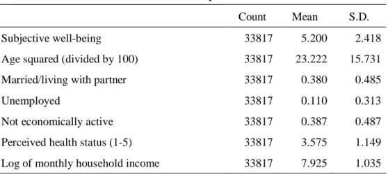
In terms of the control variables, standard time-variant variables from previous studies are included (e.g., Baetschmann et al., 2015; Ferrer-i-Carbonell and Frijters, 2004; Winkelmann and Winkelmann, 1998). In addition, spatial Durbin terms (i.e., first-order spatial lag terms) of income and unemployment are included, which correspond to the average of these variables within the same round and district without individual i. These variables are proxies for the comparison between income and unemployment rate, which are known to be important determinants of SWB at the regional level (e.g., Clark and Oswald, 1996; Ferrer-i-Carbonell, 2005; McBride, 2001; Vendrik and Woltjer, 2007; Di Tella et al., 2001; Luttmer, 2005). Table 2 provides the summary statistics of the control variables.
An important issue in the estimation of spatial econometric models is that they are structural equations due to spatial dependence, and the OLS estimators are known to be inconsistent (e.g., Anselin, 1988; LeSage and Pace, 2009). For this reason, the study employs the maximum likelihood (ML) estimation for model (1) by solving the model for 𝜖𝜖𝑖𝑖𝑖𝑖 and assuming it to be independent and identically distributed following a normal distribution. Specifically, we employ the transformation approach proposed by Lee and Yu (2010) to handle the incidental parameter problem as a result of individual fixed effects.2
However, the ML approach imposes two strict restrictions in estimation. First, estimating the model requires a balanced panel data. For this reason, the sample is restricted to a balanced panel of (i) rounds 1 and 2, (ii) rounds 1 to 3, (iii) rounds 1 to 4, and (iv) rounds 1 to 5 to fully utilize cross-sectional and time-series variations. Notably, a long panel data can suffer additional serious sample selection problems due to attrition. Second, the weight matrix is assumed to be time-invariant. Therefore, the sample should be restricted to those who did not move across districts during the sample period. However, these sample restrictions lead to a huge loss of the sample.
To complement such caveats, the entire panel data are used, and the spatial autoregressive (SAR) model with several types of fixed effects is estimated as follows:
𝑦𝑦𝑖𝑖𝑖𝑖 = 𝜌𝜌 � 𝑤𝑤𝑖𝑖𝑖𝑖𝑖𝑖𝑦𝑦𝑖𝑖𝑖𝑖 𝑁𝑁
𝑖𝑖=1
+ 𝑥𝑥𝑖𝑖𝑖𝑖𝛽𝛽 + 𝛿𝛿𝑖𝑖 + 𝜁𝜁𝑖𝑖+ 𝜙𝜙𝑑𝑑+ 𝜂𝜂𝑝𝑝𝑖𝑖 + 𝜖𝜖𝑖𝑖𝑖𝑖. (2)
A notable difference from model (1) is that weight 𝑤𝑤𝑖𝑖𝑖𝑖𝑖𝑖 is time-variant, which enables the respondent to move across districts. For this reason, district fixed effects 𝜙𝜙𝑑𝑑 can be included separately from individual fixed effects. By testing whether or not 𝜙𝜙𝑑𝑑s are jointly significant, the occurrence of regional disparities even after controlling for individual level unobserved heterogeneities can be discussed. In addition, province-round fixed effects 𝜂𝜂𝑝𝑝𝑖𝑖 are included to control for potential time-variant geographical heterogeneities.3 However, including a spatial error term is virtually impossible because of the time-variant spatial weight and unbalanced panel structure. Therefore, models (1) and (2) are characterized by their advantages and disadvantages.
2 This approach reduces the effective sample size from NT to N(T − 1).
3 Province-round fixed effects are included to avoid multicollinearity because the spatial lag
The same ML approach cannot be applied to the estimation of model (2) due to the above-mentioned issues. Instead, the instrumental variable (IV) approach is employed by using the first-order spatial lag terms of the dependent variables ∑𝑁𝑁𝑖𝑖=1𝑤𝑤𝑖𝑖𝑖𝑖𝑖𝑖𝑥𝑥𝑖𝑖𝑖𝑖 as independent variables (IVs) for the endogenous variable ∑𝑁𝑁𝑖𝑖=1𝑤𝑤𝑖𝑖𝑖𝑖𝑖𝑖𝑦𝑦𝑖𝑖𝑖𝑖. The assumption for the validity of IVs requires that the individual characteristics of neighbors will affect their SWB only and not directly affect individual i’s SWB.
In addition to individual data analysis to test for spillover effects within a district, the study investigates whether spillover effects occur in SWB across districts. For this purpose, data are collapsed into district-level by taking the average of each variable and estimating a similar model as in Equation (1):
𝑦𝑦𝑑𝑑𝑖𝑖𝑖𝑖= 𝜌𝜌 � 𝑤𝑤𝑑𝑑𝑖𝑖𝑑𝑑𝑗𝑗𝑦𝑦𝑑𝑑𝑗𝑗𝑖𝑖 𝑁𝑁 𝑖𝑖=1 + 𝑥𝑥𝑑𝑑𝑖𝑖𝑖𝑖𝛽𝛽 + 𝜁𝜁𝑖𝑖+ 𝜙𝜙𝑑𝑑𝑖𝑖+ 𝑢𝑢𝑑𝑑𝑖𝑖𝑖𝑖 (3) 𝑢𝑢𝑑𝑑𝑖𝑖𝑖𝑖 = 𝜆𝜆 � 𝑤𝑤𝑑𝑑𝑖𝑖𝑑𝑑𝑗𝑗𝑢𝑢𝑑𝑑𝑗𝑗𝑖𝑖 𝑁𝑁 𝑖𝑖=1 + 𝜖𝜖𝑑𝑑𝑖𝑖𝑖𝑖,
where the unit of observation is district-level (𝑑𝑑𝑖𝑖). As for the weight matrix, two types of matrices are used to test the robustness of the findings. The first is an inverse distance matrix, which is based on the geographical distance between 𝑑𝑑𝑖𝑖 and 𝑑𝑑𝑖𝑖. The second is a contiguity matrix whose element 𝑤𝑤𝑑𝑑𝑖𝑖𝑑𝑑𝑗𝑗 takes a value of one if 𝑑𝑑𝑖𝑖 and 𝑑𝑑𝑖𝑖 are contiguous with each other. Otherwise, it takes a value of zero. Both matrices are row-standardized such that
∑𝑁𝑁𝑖𝑖=1𝑤𝑤𝑑𝑑𝑖𝑖𝑑𝑑𝑗𝑗𝑦𝑦𝑑𝑑𝑗𝑗𝑖𝑖 is equivalent to the (weighted) average SWB over neighboring districts. By
doing so, the spatial lag term captures spillover effects across districts. 𝑥𝑥𝑑𝑑𝑖𝑖𝑖𝑖 includes the same set of control variables as in models (1) and (2) for comparison. The study utilizes the transformation approach to avoid the incidental parameter problem because the data are a strongly balanced panel.
Notably, the approach differs from those of previous studies estimating a spatial econometric model with region- or country-level data (Stanca, 2010; Lin et al., 2014; 2017) because time-invariant unobserved heterogeneities can be controlled by including district fixed effects. Previous studies have failed to incorporate fixed effects because they analyzed cross-sectional data, and the estimated coefficient may be confounded with unobserved heterogeneities. In addition, the present study enables the error term to be spatially correlated. Whether or not a significant spatial correlation exists in the error term after controlling for the
fixed effects continues to be an issue in the literature. For this purpose, the likelihood ratio test and Akaike information criterion (AIC) are employed as model selection criteria.
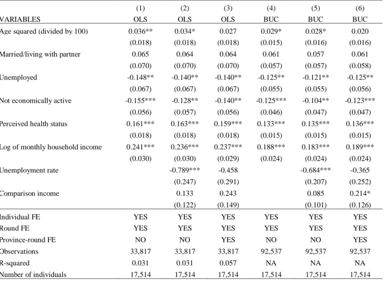
A potential threat in the estimation of models (1) to (3) is that the linear models are estimated by treating SWB as a cardinal variable, although it is actually observed as an ordinal variable. As discussed in previous studies (e.g., Ferrer-i-Carbonell and Frijters, 2004; Frey and Stutzer, 2000), employing either OLS or ordered probit/logit models are known to exert little difference in the qualitative results. To confirm this issue in the current dataset, the model is estimated by OLS, and the ordered logit model estimated using the blow-up and cluster (BUC) approach (Baetschmann et al., 2015). The estimation results are then compared. The results of the model are estimated without spatial lag or error term because the BUC approach does not allow for the inclusion of spatial terms. The comparison confirms that the qualitative results remain basically unchanged between OLS and BUC (Tables A2). Therefore, SWB is treated as a cardinal variable, and the above-mentioned liner spatial econometric model estimated.
Another potential threat of SWB regressions is the critique by Bond and Lang (2019), who argued that the econometric analysis of happiness data is dependent on strong assumptions and that the findings of previous studies can be theoretically reversible. However, Chen et al. (2019) proposed that such problems are avoidable by focusing on the median rather than the mean. Following this notion, quantile regression is estimated with individual FEs to test for the stability of the coefficients.4 Notably, this approach also does not allow for the inclusion of spatial terms, such that the model is estimated without these terms. Estimation results indicate that the point estimates are virtually unaffected, although several coefficients are less precisely estimated than OLS (Table A3). Thus, the critique by Bond and Lang (2019) may be irrelevant in the current analysis.
4. Estimation Results
4.1. Within-district Externalities
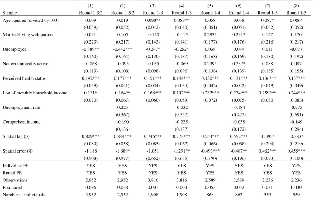
First, the spatial externalities in SWB within a district are tested by estimating model (1). Table 3 provides the estimation results with a different set of samples, i.e., the balanced panel data of the first and second rounds (columns (1) and (2)), from the first to the third rounds (columns (3) and (4)), from the first to the fourth rounds (columns (5) and (6)), and all five rounds (columns (6) and (7)).
4 Chen et al. (2019) originally proposed to employ the heteroskedastic ordered logit model.
However, the present study employs the quantile regression model to include individual fixed effects, which is difficult to incorporate in the suggested model.
The spatial lag term, which is the main parameter of interest, is significantly positive in the majority of cases, which indicates that spatial spillovers in SWB exist within a district even after controlling for individual- or district-level heterogeneities. However, the coefficient is negative and marginally significant in the last two columns using the balanced panel for all five rounds of the survey. This contradicting result may be derived from significant attrition in the sample, that is, the number of respondents was reduced from 2,952 in the panel of rounds 1 and 2 to 559 in the panel of all five rounds. This sample selection problem may lead to a biased estimate in the spatial lag term. Interestingly, the spatial error term is statistically significant in many columns, which suggests unobserved heterogeneities that are spatially correlated.
As for the controlling variables, better health condition and household income are significantly positive across specifications, which is consistent with previous studies (e.g., Clark et al., 2008; Borghesi et al., 2010). Other well-known results, such as the U-shaped effect of age (e.g., Blanchflower and Oswald, 2004), positive effect of being married (e.g., Alesina et al., 2004; Clark and Oswald, 2002; Oswald 1997), and negative effect of being unemployed (e.g. Winkelmann and Winkelmann 1998; Frey and Stutzer 2002; Blanchflower and Oswald 2004; Kingdon and Knight 2006), are also supported. However, such results are not necessarily robust in several specifications. In contrast, the study lacks significant supporting evidence for the negative effect of unemployment rate or comparison income, although the sign of the average income within a district is negative across specifications.
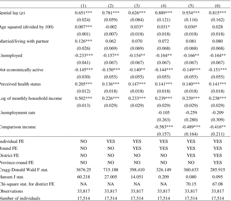
As previously mentioned, the results thus far may suffer from sample selection due to the construction of the balanced panel data and time-invariant weight matrix. For this reason, model (2) is estimated. Table 4 illustrates the results. Notably, the effective sample size is much larger than that in Table 3. The first stage F statistics rejects the null hypothesis and passes the weak instrument test in all specifications. In contrast, Hansen’s J statistics significantly rejects the null hypothesis in columns (1)–(3), which suggests that the instruments can be regarded as exogenous only after controlling for comparison income as well as individual FEs and round FEs.
Importantly, the spatial lag term is significantly positive in all specifications, which supports the spatial externalities in SWB after controlling for individual- and region-level heterogeneities. The point estimates imply that a one-point increase in the average SWB within a district corresponds to an increase of 0.63–0.93 points in own SWB. This magnitude is comparable to the ones by ML estimation (Table 3), thus confirming the robustness of the finding to the estimation methods. Furthermore, the spatial lag term remains significantly
positive after including additional controls from columns (1) to (6), which implies a certain level of robustness to the possible omitted variable bias.
In addition, the study confirms the U-shaped effect of age, the negative effect of being unemployed or economically inactive, and the positive effect of better health and high income. Intriguingly, the coefficient on the average income within a district becomes significantly negative in all specifications. This result contradicts that of Kingdon and Knight (2007), who found a positive effect of the comparison income on SWB in the South African context. This contrast may result from including the spatial lag term for SWB and controlling for individual- and region-level heterogeneities by including fixed effects.
As previously discussed, an advantage of model (2) is that district fixed effects can be incorporated separately from individual fixed effects. These district fixed effects are jointly significant in columns (3) and (4), which suggests that regional level heterogeneities in SWB remain after controlling for observed and unobserved individual characteristics. This finding implies that region-level heterogeneities, as well as spatial externalities, are essential drivers of regional disparities in SWB.
4.2. Across-district Externalities
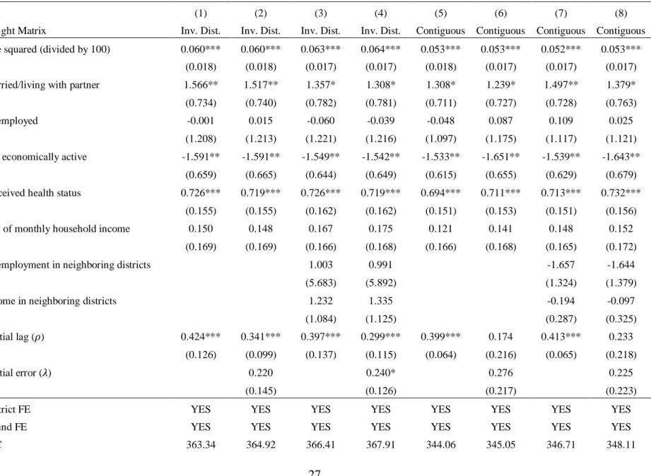
At this point, the study analyzes district-level data to test for spatial externalities in SWB across districts. For this purpose, data are collapsed from the individual to district-level panel data. As a result, strictly balanced panel data of five survey rounds are obtained. Using these data, the spatial econometric model specified in Equation (3) is estimated. Table 5 shows the estimation results, where columns (1) to (4) pertain to the estimation results with the inverse distance matrix, whereas columns (5) to (8) denote the results with the contiguity matrix.
Consistent with the individual panel data analysis, the coefficients on the district averages of age squared, being economically inactive, and better health condition have the same sign and are highly significant. In contrast, the shares for being unemployed and average income are insignificant. The coefficients on these variables are robust across specifications. The main parameter of interest, namely, the spatial lag term for the average SWB, is significantly positive in the majority of specifications. Although it becomes insignificant when the spatial error term 𝜆𝜆 is included with the contiguity weight matrix, 𝜆𝜆 is statistically insignificant by itself, and neither the LR test nor AIC supports its inclusion. Therefore, the preferred model is SAR, and significant spatial externalities in SWB are confirmed.
The point estimates imply that a one-point increase in the (weighted) average SWB over neighboring districts correspond to an increase of 0.30–0.42 points in district i’s average SWB. This finding is robust to the choice of the weight matrix. In addition, this magnitude is
relatively smaller compared with those of Stanca (2010) and Lin et al. (2017), which possibly implies confoundedness in the estimated spatial lag term with unobserved region-level heterogeneities as observed in the previous studies. Indeed, the estimation results of the same model without district fixed effects confirm the high magnitudes of the spatial lag and spatial error terms (Table A4).
5. Conclusion
Previous studies have shown regional disparities in SWB, which is robust to the control of individual characteristics. This phenomenon can be explained by region-level heterogeneities and spatial externalities in SWB. However, the two factors frequently confound each other, and testing for externalities after controlling for region-level heterogeneities remains an important issue to be investigated.
Using a nationally representative household survey data in South Africa, the current study estimates spatial econometric versions of SWB regression. Estimation results show significantly positive spatial externalities in SWB within a district at the individual level and across districts at the district-level. To the best of the authors’ knowledge, this study is one of the first to find a significant spatial spillover effect in SWB by explicitly controlling for region-level heterogeneities. Within-district externality is relatively high: a one-point increase in the average SWB within a district corresponds to an increase of 0.63–0.93 points in its SWB. In contrast, analysis of across-district externality at the district-level indicates that the magnitude of the coefficient of the spatial lag term is smaller, although significant, than those of previous studies. This finding implies that previous estimates may be confounded by unobserved heterogeneities.
Distinguishing within-district spillover from district-level heterogeneities has an important policy implication. The existence of district-level heterogeneities implies that improving institutions and amenities leads to the high levels of SWB of individuals living in a district. In contrast, within-district spillover justifies policy intervention targeting a specific group of people within a district because improving SWB leads to the high levels of SWB of the surrounding people unless the intervention aggravates the welfare of these non-targeted individual.
Moreover, results indicate that spatial econometrics is an effective approach for testing the spillover effect of SWB within and across regional clusters. However, the estimated impact notably does not necessarily indicate the causal effect of the SWB of the neighbor on his/her SWB due to the reflection problem (Manski, 1993). Rather, the main interest of the
study lies in the existence of spillover in SWB, which is an equilibrium of the reflection effect between the two variables. Therefore, testing for a strict causal relationship remains an important issue that future research should explore.
Funding: The research was supported by Japan Society for the Promotion of Science
KAKENHI Grant Numbers 16H00739 and 18K12786.
Acknowledgements: I am grateful to Kyoji Fukao, Takahiro Fukunishi, Nobuyoshi Kikuchi,
Yasumasa Matsuda, Takeshi Murooka, Hitoshi Sato, Takaki Sato, Masahiro Shoji, Shoko Yamane, and the participants at SEA 2018, ABEF 2019, and the seminar at CDRI. All remaining errors are my own.
Reference
Agüero, J., Carter, M. R., May, J., 2007. Poverty and Inequality in the First Decade of South Africa’s Democracy: What can be Learnt from Panel Data from KwaZulu-Natal? Journal of African Economies 16(5), 782–812.
Aida, T., 2018. Exploring the Relationship between Subjective Well-Being and Objective Poverty Indices: Evidence from Panel Data in South Africa. IDE Discussion Papers No.707.
Alesina, A., Di Tella, R., MacCulloch, R., 2004. Inequality and Happiness: Are Europeans and Americans different? Journal of Public Economics. 88(9–10), 2009–42.
Anselin, L., 1988. Spatial Econometrics: Methods and Models. Dordrecht, The Netherlands: Kluwer Academic Publishers.
Aslam, A., Corrado, L., 2012. The geography of well-being. Journal of Economic Geography 12, 627–649.
Baetschmann, G., Staub, K. E., Winkelmann, R., 2015. Consistent estimation of the fixed effects ordered logit model. Journal of the Royal Statistical Society, Statistics in Society, Series A 178(3), 685–703.
Ballas, D., Tranmer, M., 2012. Happy people or happy places? A multilevel modeling approach to the analysis of happiness and well-being. International Regional Science Review 35(1), 70-102.
Blanchflower, D. G., Oswald, A. J., 2004. Well-being over time in Britain and the USA. Journal of Public Economics 88(7–8), 1359–86.
Bond, T. N., Lang, K., 2019. The Sad Truth about Happiness Scales. Journal of Political Economy 127(4), 1629-1640.
Borghesi, S., Vercelli, A., 2010. Happiness and Health: Two Paradoxes. Journal of Economic Surveys 26(2), 203–233.
Bosker, M., Krugell, W., 2008. Regional Income Evolution in South Africa after Apartheid. Journal of Regional Science 48(3), 493–523.
Brereton, F., Clinch, J. P., Ferreira, S., 2008. Happiness, geography and the environment. Ecological Economics 65, pp. 386–396.
Carter, M. R., May, J., 2001. One Kind of Freedom: Poverty Dynamics in Post-apartheid South Africa. World Development 29(12), 1987–2006.
Chen, L.-Y., Oparina, E., Powdthavee, N., Srisuma, S., 2019. Have Econometric Analyses of Happiness Data Been Futile? A Simple Truth about Happiness Scales. IZA DP No. 12152
Clark, A. E., Frijters, P., Shields, M. A., 2008. Relative Income, Happiness, and Utility: An Explanation for the Easterlin Paradox and Other Puzzles. Journal of Economic Literature 46(1), 95-144
Clark, A. E., Oswald, A. J., 1996. Satisfaction and comparison income. Journal of Public Economics 61(3), 359–381.
Clark, A. E., Oswald, A. J., 2002. A simple statistical method for measuring how life events affect happiness. International Journal of Epidemiology 31(6), 1139–1144.
Christopher, A. J., 1992. Segregation Levels in South African Cities, 1911-1985. International Journal of African Historical Studies 25(3), 561-582
David, A., Guilbert, N., Hamaguchi, N., Higashi, Y., Hino, H., Leibbrandt M., Shifa, M., 2018. Spatial poverty and inequality in South Africa: A municipality level analysis. SALDRU Working Paper Number 221.
Di Tella, R., MacCulloch, R. J., Oswald, A. J., 2001. Preferences over Inflation and Unemployment: Evidence from Surveys of Happiness. American Economic Review 91(1), 335-341.
Dolan, P., Peasgood, T., White, M., 2008. Do we really know what makes us happy? A review of the economic literature on the factors associated with subjective well-being. Journal of Economic Psychology 29, 94–122.
Easterlin, R. E., 1974. Does economic growth improve the human lot? Some empirical evidence, in: David, P.A., Reder, M.W. (Eds.), Nations and Households in Economic Growth: Essays in Honour of Moses Abramowitz. Academic Press, New York.
Ferrer-i-Carbonell, A., 2005. Income and well-being: An empirical analysis of the comparison income effect. Journal of Public Economics 89(5–6), 997–1019.
Ferrer-i-Carbonell, A., Frijters, P., 2004. How Important Is Methodology for The Estimates of The Determinants of Happiness? Economic Journal 114, 641–659.
Finn, A., Leibbrandt, M., 2016. The dynamics of poverty in the first four waves of NIDS. SALDRU Working Paper Number 174/ NIDS Discussion Paper 2016/1.
Fowler, J., Christakis, N., 2008. Dynamic spread of happiness in a large social network: longitudinal analysis over twenty years in the Framingham heart study. British Medical Journal 337, pp. 2338.
Frey, B. S., Stutzer, A., 2000. Happiness, economy and institutions. Economic Journal 110: 918–938.
Frey, B. S., Stutzer, A. 2002. What Can Economists Learn from Happiness Research? Journal of Economic Literature 40(2), 402-435.
Gradin, C., 2012. Race, Poverty and Deprivation in South Africa. Journal of African Economies 22(2), 187–238.
Hogan, M. J., Leyden, K. M., Conway, R., Goldberg, A., Walsh, D., McKenna-Plumley, P. E., 2016. Happiness and health across the lifespan in five major cities: The impact of place and government performance. Social Science & Medicine 162, 168–176.
Kingdon, G. G., Knight, J., 2006. Subjective well-being poverty vs. Income poverty and capabilities poverty? Journal of Development Studies 42(7), 1199–1224.
Kingdon, G. G., Knight, J., 2007. Community comparisons and subjective well-being in a divided society. Journal of Economic Behavior & Organization, 64, 69–90.
Leibbrandt, M., Woolard, I., 1999. A comparison of poverty in South Africa's nine provinces. Development Southern Africa 16(1), 37-54.
LeSage, J., Pace, R. K., 2009. Introduction to Spatial Econometrics. Boca Raton: Taylor & Francis.
Lee, L-f, Yu, J. 2010. Estimation of spatial autoregressive panel data models with fixed effects. Journal of Econometrics 154, 165–185.
Lin, C. A., Lahiri, S., Hsu, C. P., 2014. Happiness and Regional Segmentation: Does Space Matter? Journal of Happiness Studies 15, 157–183.
Lin, C.-H. A., Lahiri, S., Hsu, C.-P., 2017. Happiness and Globalization: A Spatial Econometric Approach. Journal of Happiness Studies 18(6), 1841–1857.
Luttmer, E.F.P., 2005. Neighbors as negatives: relative earnings and well-being. Quarterly Journal of Economics 120(3), 963–1002.
MacKerron, G., 2012. Happiness Economics from 35 000 Feet. Journal of Economic Surveys 26(4), 705–735.
Manski, C. F., 1993. Identification of endogenous social effects: The reflection problem. Review of Economic Studies 60, 531–542.
McBride, M., 2001. Relative-income effects on subjective well-being in the cross-section. Journal of Economic Behavior & Organization 45(3), 251–278.
Neff, D. F., 2007. Subjective Well-Being, Poverty and Ethnicity in South Africa: Insights from an Exploratory Analysis. Social Indicators Research 80, 313–341.
Oswald, A. J., 1997. Happiness and economic performance. Economic Journal 107(445), 1815–31.
Oswald, A. J., Wu, S., 2011. Well-Being across America. Review of Economics and Statistics 93(4), 1118–1134.
Pittau, M. G., Zelli, R., Gelman, A., 2010. Economic Disparities and Life Satisfaction in European Regions. Social Indicators Research 96, 339–361.
Posel, D., 2004. Have Migration Patterns in Post-Apartheid South Africa Changed? Journal of Interdisciplinary Economics 15, 277–292.
Powdthavee, N., 2005. Unhappiness and Crime: Evidence from South Africa. Economica 72, 531–547.
Powdthavee, N., 2007. Are There Geographical Variations in The Psychological Cost of Unemployment in South Africa? Social Indicators Research 80, 629–652.
Stanca, L., 2010. The Geography of Economics and Happiness: Spatial Patterns in the Effects of Economic Conditions on Well-Being. Social Indicator Research 99, 115–133.
Stiglitz, J. E., Sen, A., Fitoussi, J., 2009. Report by the Commission on the Measurement of Economic Performance and Social Progress, Commission on the Measurement of Economic Performance and Social Progress, Paris.
Tumen, S., Zeydanli, T., 2015. Is happiness contagious? Separating spillover externalities from the group-level social context. Journal of Happiness Studies 16(3):1–26.
Vendrik, M. C.M., Woltjer, G. B., 2007. Happiness and loss aversion: Is utility concave or convex in relative income? Journal of Public Economics 91(7–8),1423–1448.
Winkelmann, L., Winkelmann, R., 1998. Why are the Unemployed So Unhappy? Evidence from Panel Data. Economica 65(257), 1–15.
Table 1: Moran’s I Statistics for Subjective Well-being by Survey Round
Panel A: Within-district externalities (Individual Level) Moran’s I S.D. Round 1 0.118*** 0.002 Round 2 0.142*** 0.002 Round 3 0.116*** 0.001 Round 4 0.075*** 0.001 Round 5 0.075*** 0.001 Panel B: Across-district externalities (District Level)
Moran’s I S.D. Round 1 0.175*** 0.022 Round 2 0.135*** 0.022 Round 3 0.15*** 0.022 Round 4 0.135*** 0.022 Round 5 0.087*** 0.022
Table 2: Summary Statistics
Count Mean S.D. Subjective well-being 33817 5.200 2.418 Age squared (divided by 100) 33817 23.222 15.731 Married/living with partner 33817 0.380 0.485 Unemployed 33817 0.110 0.313 Not economically active 33817 0.387 0.487 Perceived health status (1-5) 33817 3.575 1.149 Log of monthly household income 33817 7.925 1.035
Table 3: Estimation Result of Spatial Econometric Model with Balanced Panel
(1) (2) (3) (4) (5) (6) (7) (8)
Sample Round 1 &2 Round 1 &2 Round 1-3 Round 1-3 Round 1-4 Round 1-4 Round 1-5 Round 1-5 Age squared (divided by 100) 0.009 0.019 0.090** 0.089** 0.058 0.058 0.087* 0.086*
(0.059) (0.052) (0.042) (0.040) (0.051) (0.051) (0.052) (0.052) Married/living with partner 0.091 0.105 -0.120 -0.115 0.293* 0.291* 0.167 0.170
(0.223) (0.217) (0.143) (0.141) (0.177) (0.176) (0.216) (0.217) Unemployed -0.389** -0.442*** -0.247* -0.252* 0.038 0.049 0.011 -0.077 (0.160) (0.164) (0.130) (0.137) (0.168) (0.169) (0.180) (0.192) Not economically active -0.068 -0.095 -0.055 -0.069 0.239* 0.237* 0.088 0.087
(0.113) (0.108) (0.098) (0.096) (0.138) (0.139) (0.155) (0.155) Perceived health status 0.192*** 0.177*** 0.151*** 0.144*** 0.130*** 0.131*** 0.136*** 0.137***
(0.039) (0.041) (0.034) (0.034) (0.042) (0.042) (0.049) (0.049) Log of monthly household income 0.131* 0.164** 0.166*** 0.192*** 0.232*** 0.234*** 0.259*** 0.244***
(0.070) (0.067) (0.060) (0.059) (0.072) (0.075) (0.080) (0.083) Unemployment rate 0.225 -0.032 -0.184 -0.975 (0.367) (0.327) (0.422) (0.691) Comparison income -0.190 -0.225 -0.038 -0.149 (0.136) (0.137) (0.172) (0.294) Spatial lag (𝜌𝜌) 0.809*** 0.844*** 0.746*** 0.773*** 0.554*** 0.552*** -0.395* -0.383* (0.080) (0.058) (0.085) (0.067) (0.066) (0.068) (0.204) (0.219) Spatial error (𝜆𝜆) -1.188 -1.689* -1.051 -1.291** -0.493*** -0.487** 0.462*** 0.455*** (0.908) (0.977) (0.652) (0.635) (0.190) (0.196) (0.093) (0.100)
Individual FE YES YES YES YES YES YES YES YES
Round FE YES YES YES YES YES YES YES YES
Observations 2,952 2,952 3,816 3,816 2,589 2,589 2,236 2,236
R-squared 0.096 0.038 0.001 0.000 0.053 0.052 0.031 0.030
Table 4: Estimation Result of Spatial Econometric Model with Unbalanced Panel
(1) (2) (3) (4) (5) (6)
Spatial lag (𝜌𝜌) 0.651*** 0.781*** 0.626*** 0.889*** 0.934*** 0.815*** (0.024) (0.059) (0.084) (0.121) (0.116) (0.162) Age squared (divided by 100) 0.007*** -0.002 0.033* 0.031* 0.030* 0.028
(0.001) (0.007) (0.018) (0.018) (0.018) (0.018) Married/living with partner 0.126*** 0.062 0.070 0.072 0.081 0.080
(0.026) (0.069) (0.069) (0.068) (0.068) (0.068) Unemployed -0.233*** -0.157** -0.154** -0.164** -0.166** -0.164**
(0.041) (0.067) (0.067) (0.067) (0.067) (0.067) Not economically active -0.145*** -0.150*** -0.140** -0.144*** -0.149*** -0.151***
(0.030) (0.055) (0.055) (0.055) (0.055) (0.055) Perceived health status 0.205*** 0.136*** 0.147*** 0.141*** 0.140*** 0.141***
(0.012) (0.018) (0.018) (0.018) (0.018) (0.018) Log of monthly household income 0.502*** 0.226*** 0.233*** 0.239*** 0.239*** 0.238***
(0.013) (0.029) (0.029) (0.029) (0.029) (0.029)
Unemployment rate -0.105 -0.259 -0.209
(0.263) (0.280) (0.309)
Comparison income -0.583*** -0.489*** -0.416**
(0.157) (0.164) (0.211)
Individual FE NO YES YES YES YES YES
Round FE NO NO YES YES YES YES
District FE NO NO NO NO YES YES
Province-round FE NO NO NO NO NO YES
Cragg-Donald Wald F stat. 3676.25 715.188 398.410 326.149 360.633 285.915 Hansen J stat. 60.218 27.005 14.051 0.209 0.080 0.095 Chi-square stat. for district FE NA NA NA NA 70.15 67.08 Observations 33,817 33,817 33,817 33,817 33,817 33,817 Number of individuals 17,514 17,514 17,514 17,514 17,514 17,514
Note: Robust standard errors at individual level are in parentheses. *** p < 0.01, ** p < 0.05, * p < 0.1.
Table 5: Estimation Result of Spatial Econometric Model with District Panel
(1) (2) (3) (4) (5) (6) (7) (8)
Weight Matrix Inv. Dist. Inv. Dist. Inv. Dist. Inv. Dist. Contiguous Contiguous Contiguous Contiguous Age squared (divided by 100) 0.060*** 0.060*** 0.063*** 0.064*** 0.053*** 0.053*** 0.052*** 0.053***
(0.018) (0.018) (0.017) (0.017) (0.018) (0.017) (0.017) (0.017) Married/living with partner 1.566** 1.517** 1.357* 1.308* 1.308* 1.239* 1.497** 1.379* (0.734) (0.740) (0.782) (0.781) (0.711) (0.727) (0.728) (0.763) Unemployed -0.001 0.015 -0.060 -0.039 -0.048 0.087 0.109 0.025
(1.208) (1.213) (1.221) (1.216) (1.097) (1.175) (1.117) (1.121) Not economically active -1.591** -1.591** -1.549** -1.542** -1.533** -1.651** -1.539** -1.643**
(0.659) (0.665) (0.644) (0.649) (0.615) (0.655) (0.629) (0.679) Perceived health status 0.726*** 0.719*** 0.726*** 0.719*** 0.694*** 0.711*** 0.713*** 0.732***
(0.155) (0.155) (0.162) (0.162) (0.151) (0.153) (0.151) (0.156) Log of monthly household income 0.150 0.148 0.167 0.175 0.121 0.141 0.148 0.152
(0.169) (0.169) (0.166) (0.168) (0.166) (0.168) (0.165) (0.172)
Unemployment in neighboring districts 1.003 0.991 -1.657 -1.644
(5.683) (5.892) (1.324) (1.379)
Income in neighboring districts 1.232 1.335 -0.194 -0.097
(1.084) (1.125) (0.287) (0.325)
Spatial lag (𝜌𝜌) 0.424*** 0.341*** 0.397*** 0.299*** 0.399*** 0.174 0.413*** 0.233 (0.126) (0.099) (0.137) (0.115) (0.064) (0.216) (0.065) (0.218)
Spatial error (𝜆𝜆) 0.220 0.240* 0.276 0.225
(0.145) (0.126) (0.217) (0.223)
District FE YES YES YES YES YES YES YES YES
Round FE YES YES YES YES YES YES YES YES
Likelihood ratio test for 𝜆𝜆 0.414 0.50 1.01 0.06
Observations 208 208 208 208 208 208 208 208
R-squared 0.363 0.360 0.387 0.387 0.365 0.355 0.356 0.357
Number of districts 52 52 52 52 52 52 52 52
Table A1: Results for Regression Adjusted Subjective Well-Being at District Level
(1)
Age squared (divided by 100) 0.0345*** (0.00461) Married/living with partner 0.146*** (0.0289)
Unemployed -0.276***
(0.0422) Not economically active -0.169***
(0.0320) Perceived health status 0.209***
(0.0123) Log of monthly household income 0.391***
(0.0156) Age -0.0238*** (0.00457) Race = Coloured 0.804*** (0.0562) Race = Asian/Indian 0.935*** (0.117) Race = White 0.945*** (0.0610) Female 0.0258 (0.0268) Education = Foundation 0.280*** (0.0661) Education = Intermediate 0.191*** (0.0499) Education = Senior 0.281*** (0.0471) Education = National senior certificate 0.419***
(0.0492) Education = Above 0.539*** (0.0558) Round FE YES District FE YES Observations 33,701 R-squared 0.163
Note: Robust standard errors at individual level are in parentheses. *** p < 0.01, ** p < 0.05, * p < 0.1.
Table A2: Comparison between OLS and Ordered Logit Model (BUC)
(1) (2) (3) (4) (5) (6)
VARIABLES OLS OLS OLS BUC BUC BUC
Age squared (divided by 100) 0.036** 0.034* 0.027 0.029* 0.028* 0.020 (0.018) (0.018) (0.018) (0.015) (0.016) (0.016) Married/living with partner 0.065 0.064 0.064 0.061 0.057 0.061
(0.070) (0.070) (0.070) (0.057) (0.057) (0.058) Unemployed -0.148** -0.140** -0.140** -0.125** -0.121** -0.125**
(0.067) (0.067) (0.067) (0.055) (0.055) (0.056) Not economically active -0.155*** -0.128** -0.140** -0.125*** -0.104** -0.123***
(0.056) (0.057) (0.056) (0.046) (0.047) (0.047) Perceived health status 0.161*** 0.163*** 0.159*** 0.133*** 0.135*** 0.136***
(0.018) (0.018) (0.018) (0.015) (0.015) (0.015) Log of monthly household income 0.241*** 0.236*** 0.237*** 0.188*** 0.183*** 0.189***
(0.030) (0.030) (0.029) (0.024) (0.024) (0.024) Unemployment rate -0.789*** -0.458 -0.684*** -0.365 (0.247) (0.291) (0.207) (0.252)
Comparison income 0.133 0.243 0.085 0.214*
(0.122) (0.149) (0.101) (0.126)
Individual FE YES YES YES YES YES YES
Round FE YES YES YES YES YES YES
Province-round FE NO NO YES NO NO YES
Observations 33,817 33,817 33,817 92,537 92,537 92,537
R-squared 0.031 0.031 0.057 NA NA NA
Number of individuals 17,514 17,514 17,514 17,514 17,514 17,514
Note: Robust standard errors at individual level are in parentheses. *** p < 0.01, ** p < 0.05, * p < 0.1.
Table A3: Comparison between OLS and Quantile Regression Model
(1) (2) (3) (4) (5) (6)
VARIABLES OLS OLS OLS Quantile Quantile Quantile
Age squared (divided by 100) 0.036** 0.034* 0.027 0.036 0.034 0.027 (0.018) (0.018) (0.018) (0.027) (0.074) (0.050) Married/living with partner 0.065 0.064 0.064 0.064 0.063 0.062
(0.070) (0.070) (0.070) (0.103) (0.277) (0.187) Unemployed -0.148** -0.140** -0.140** -0.147 -0.139 -0.138 (0.067) (0.067) (0.067) (0.100) (0.269) (0.182) Not economically active -0.155*** -0.128** -0.140** -0.156* -0.129 -0.141 (0.056) (0.057) (0.056) (0.082) (0.222) (0.150) Perceived health status 0.161*** 0.163*** 0.159*** 0.160*** 0.163** 0.158***
(0.018) (0.018) (0.018) (0.027) (0.071) (0.048) Log of monthly household income 0.241*** 0.236*** 0.237*** 0.242*** 0.237** 0.238***
(0.030) (0.030) (0.029) (0.043) (0.116) (0.079)
Unemployment rate -0.789*** -0.458 -0.778 -0.445
(0.247) (0.291) (0.985) (0.792)
Comparison income 0.133 0.243 0.135 0.243
(0.122) (0.149) (0.496) (0.408)
Individual FE YES YES YES YES YES YES
Round FE YES YES YES YES YES YES
Province-round FE NO NO YES NO NO YES
Observations 33,817 33,817 33,817 33,817 33,817 33,817
R-squared 0.031 0.031 0.057 NA NA NA
Number of individuals 17,514 17,514 17,514 17,514 17,514 17,514
Note: Robust standard errors at individual level are in parentheses. *** p < 0.01, ** p < 0.05, * p < 0.1.
Table A4: Estimation Result of Spatial Econometric Model with District Panel (without Individual Fixed Effects)
(1) (2) (3) (4) (5) (6) (7) (8)
Weight Matrix Inv. Dist. Inv. Dist. Inv. Dist. Inv. Dist. Contiguous Contiguous Contiguous Contiguous Age squared (divided by 100) 0.048*** 0.052*** 0.048*** 0.052*** 0.043*** 0.049*** 0.042** 0.049***
(0.018) (0.018) (0.018) (0.018) (0.016) (0.017) (0.016) (0.016) Married/living with partner 1.579*** 1.326** 1.113* 0.892 1.186** 1.398** 1.305** 1.284** (0.604) (0.620) (0.639) (0.646) (0.567) (0.609) (0.580) (0.627) Unemployed -0.900 -0.908 -0.795 -0.859 -0.889 -0.882 -0.830 -0.988 (0.934) (0.929) (0.942) (0.925) (0.864) (0.895) (0.878) (0.929) Not economically active -2.012*** -2.070*** -1.726*** -1.810*** -1.722*** -2.026*** -1.789*** -1.965***
(0.509) (0.509) (0.524) (0.520) (0.474) (0.537) (0.485) (0.514) Perceived health status 0.223 0.294* 0.189 0.270 0.293* 0.397** 0.310** 0.455***
(0.170) (0.173) (0.172) (0.174) (0.158) (0.188) (0.158) (0.169) Log of monthly household income 0.323** 0.303** 0.352** 0.355*** 0.247* 0.253** 0.253** 0.305** (0.137) (0.133) (0.137) (0.134) (0.128) (0.126) (0.127) (0.128) Unemployment in neighboring districts -2.129 -1.522 -0.820 -1.729
(6.145) (6.803) (1.437) (1.861)
Income in neighboring districts 1.251** 1.413** -0.139 0.307
(0.587) (0.642) (0.173) (0.254) Spatial lag (𝜌𝜌) 0.762*** 0.676*** 0.705*** 0.577*** 0.499*** 0.281 0.517*** -0.071 (0.097) (0.131) (0.119) (0.170) (0.057) (0.245) (0.062) (0.229) Spatial error (𝜆𝜆) 0.559*** 0.571*** 0.318 0.606*** (0.181) (0.179) (0.285) (0.153) District FE NO NO NO NO NO NO NO NO
Round FE YES YES YES YES YES YES YES YES
Likelihood ratio test for 𝜆𝜆 6.027 6.415 1.380 2.736
Observations 208 208 208 208 208 208 208 208
Number of districts 52 52 52 52 52 52 52 52