NUMERICAL ANALYSIS OF UNSTEADY MOTION OF A RAREFIED GAS CAUSED BY SUDDEN CHANGE OF WALL TEMPERATURE WITH SPECIAL INTEREST IN THE PROPAGATION OF DISCONTINUITY IN THE VELOCITY DISTRIBUTION FUNCTION(Mathematical Analysis of Phenomena in Fluid and Plasma Dyna

232

NUMERICAL ANALYSIS OF UNSTEADY MOTION OF A RAREFIED GAS

CAUSED BY SUDDEN CHANGE OF WALL TEMPERATURE

WITH SPECIAL INTEREST IN THE PROPAGATION OF DISCONTINUITY

IN THE VELOCITY DISTRIBUTION FUNCTION

Kazuo Aoki, Yoshio Sone, Kenji Nishino, and Hiroshi Sugimoto

(青木一生, 曾根良夫, 西野健司, 杉元宏)

Departiuent of Aeronautical Engineering, Kyoto University, Kyoto 606, Japan

(京大・工・航空)

An unsteady gas motion induced in asemi-infinite expanse ofa rarefiedgas by

sudden beating(orcooling)of the planewallbounding thegasis analyzednunlerically

on the basis of tlie Boltzmann-Krook-Welander equation and tbe diffuse reflection. The time development of the disturbance in thegas is pursued, for variouscases of heating and cooling, over a long time from the initial moment wben $tl\iota e$ beating or

cooling occurs. In particular, thepropagation $and_{J}’\prime attenuation$of the discontinuityin $\backslash )$

the velocity distribution function are analyzed accurately.

I. INTRODUCTION

Consider a semi-infinite expanse of a rarefied gas in a uniform equilibrium state at rest,

bounded by a plane solid wall. Provided tbat tbe wall temperature changes suddenly, a gas

motion is induced owing to expansion or contraction of tlie gas by beating or cooling and the

disturbancespropagateintothegas. $Tl\iota is$simpleinitial and boundary value problemisof physical

interest because it exhibits the fundamental feature of the transition from the free molecular to

thecontinuum beliavior of tbe gas. For a small temperature change, asystematic analysis based

on the linearizedequation was carried out, and analytical resultsfor short and long time behavior

were

obtained.1

For alarge temperature change, the problem was studied by a $momel\iota tnlet1_{1}od$, but tbe result $sl_{1}owed$some unphysical

behavior.2

In the present study, we will carry out an accurate numerical allalysis of $t1_{1}e$ problem for

arbitrary temperature changes to obtain the behavior of the gas precisely over a long time from the initial moment when the wall temperature changes, $wit1_{1}$ special $e\ln$_])$1\iota asis$ on tbe following

point. In the present problem, tbe velocity distribution function is discontinuous on the wall at

the initial moment, and the discontinuity propagates into $tl\iota e$ gas, decaying owing to molecular

collisions. This situationcannot be described correctly by the standard $fi_{1l}ite- differellcemet1_{1}od$,

such as used in Refs. 3-5. $\ln t1_{1}e$ recent study of unsteady strong evaporation form a plane

condensed

phase,6,7

Sone and Sugimotodeveloped a numerical method (finite-difference method

on thecharacteristiccoordinates)describing the$disco^{c}\overline{n}tinuity$ in the velocity distribution function

correctly. On the basis oftlteir idea, we try to construct a more e{Iicient $1net1_{1}od$ to capture tbe

behavior ofthediscontinuity.

II. PROBLEM AND BASIC EQUATION

Problem: Consider a semi-infinite expanse of a rarefied

gas

($X_{1}>0,$ $X;$: rectangular space

coordinates) in contact with a stationary plane wall ($X_{1}=0$, teniperature$T_{0}$) and in a uniform

equilibrium state atrest (temperature$T_{0}$, pressure$p_{0}$). Supposethattbe wall$telnperaturec1_{1aI1}ges$

discontinuously to another uniform temperature $T_{1}$ at time$t=0$ and is kept at $T_{1}$ for all$t>0$

.

Investigate the unsteady behavior of tliegas for$t>0$ on the basis ofthe kinetic theory.

We analyze the problem under the following assumptions: (i)Tbe behavior of$t1_{1}e$ gas is

de-scribed by the $Bolt_{Z1}nann$

-itrook-Welander

equation; (ii)Thegas molecules are reflected diffusely

on tbe wall.

The Boltzmann-Krook-Welander equation in the present $s_{1)atia1[y}$ one-dimensional case is

written in thefollowingform.

数理解析研究所講究録 第 745 巻 1991 年 232-241

233

$\frac{\partial f}{\partial t}+\xi_{1}\frac{\partial f}{\partial X_{1}}=A_{c}\rho(f_{e}-f)$, (1)

$f_{e}= \frac{\rho}{(2\pi RT)^{3/2}}\exp(-\frac{(\xi_{1}-v_{1})^{2}+\xi_{2}^{2}+\xi_{3}^{2}}{2RT}))$ (2)

$\rho=\int fd\xi_{1}d\xi_{2}d\xi_{3}$, $v_{1}= \frac{1}{\rho}\int\xi_{1}fd\xi_{1}d\xi_{2}d\xi_{3}$,

(3)

$T= \frac{1}{3R\rho}\int[(\xi_{1}-v_{1})^{2}+\xi_{2}^{2}+\xi_{3}^{2}]fd\xi_{1}d\xi_{2}d\xi_{3}$, $p=R\rho T$,

where $f(X_{1}, t, \xi_{i})$ is the velocity distribution function, $\xi$; is the molecular velocity, $\rho(X_{1}, t)$ is the

gas density, $v_{i}(X_{1},t)=(v_{1}(X_{1}, t),$$0,0$) is the gas flow velocity, $T(X_{1}, t)$ is the gas temperature, $p(X_{1}, t)$ is the gas pressure, $R$ is the gas constant per unit $1\Pi ass$,

A.

is a constant ($A_{c}\rho$ is the

collision frequency of the gasmolecules), and tlie domain ofintegration is the wbole space of$\epsilon:$

.

Thediffuse-reflection boundary condition on the wall is

$f= \frac{\sigma}{(2\pi RT_{1})^{3/2}}\exp(-\frac{\xi_{i}^{2}}{2RT_{1}}I$ , for$\xi_{1}>0$, at$X_{1}=0$, (4)

where

$\sigma=-(\frac{2\pi}{RT_{1}})’$

.

$\int_{\zeta_{1}<0}\xi_{1}f(0, t, \xi_{i})d\xi_{1}d\xi_{2}d\xi_{3}$

.

(5)

$T1_{1}e$ boundary condition at infinity and $t1_{1}e$initial condition are

$f= \frac{\rho_{0}}{(2\pi lll_{0})^{3/2}}\exp(-\frac{\xi_{1}^{2}}{21ll_{0}^{1}})$ , (for$\xi_{1}<0,$ $i\backslash sX_{1}arrow\infty$) an$d$ (for all$\xi;$, at $t=0$), (6)

$w1_{1}ere\rho_{0}=p_{0}(RT_{0})^{-1}$ is$t1_{1}e$ gasdensity at the initial state.

According to Ref. 8, we can reduce the system (1)$-(6)$ to that for $g$ and $h$ defined below,

where $\xi_{2}$ and $\xi_{3}$ are eliminated. Tbat is, with $\Phi(x, t^{-}, \zeta)=[g,$$h\#$, the basic equation (1) witb (2),

(3) is reduced to

$\frac{\partial\Phi}{\partial\overline{t}}+\zeta\frac{\partial\Phi}{\partial x}=\frac{2}{\sqrt{\pi}}\frac{\rho}{\rho_{0}}(\Psi-\Phi)$ , (7)

$\Psi(M, \zeta)=[1,$ $\frac{T}{2_{O}^{1}}I\frac{1}{\sqrt{\pi}}\frac{\rho}{\rho_{0}}(\frac{T}{2_{0}^{1}})^{-1/2}\exp(-(\zeta-\frac{v_{1}}{(21l’1_{0})^{1/2}})^{2}(\frac{T}{2_{0}^{1}})^{-1}),$ (8)

$M(x,$$t \gamma=[\frac{\rho}{\rho_{0}}$ $\frac{v_{1}}{(2RT_{O})^{1/2}}\frac{T}{2_{O}^{\urcorner}}I$ ,

$\cdot$

$\frac{\rho}{\rho_{0}}=\int_{-\infty}^{\infty}gd\zeta$, $\frac{v_{1}}{(2RT_{0})^{1/2}}=(\frac{\rho}{p_{0}})^{-1}\int_{-\infty}^{\infty}\zeta gd\zeta$, (9)

$\frac{T}{T_{0}}=\frac{2}{3}(\frac{\rho}{\rho_{0}})^{-1}\{\int_{-\infty}^{\infty}(\zeta-\frac{v_{1}}{(2RT_{0})^{1/2}})^{2}gd\zeta+\int_{-\infty}^{\infty}hd\zeta\}$,

where

$g(x, \overline{t}, \zeta)=(2RT_{0})^{1/2}\rho_{0}^{-1}\iint_{-\infty}^{\infty}f(X_{1},t, \xi_{i})d\xi_{2}d\xi_{3}$,

$h(x, \overline{t}, \zeta)=(2RT_{0})^{-1/2}p_{0}^{-1}\iint_{-\infty}^{\infty}(\xi_{2}^{2}+\xi_{3}^{2})f(X_{1}, t, \xi_{i})d\xi_{2}d\xi_{3}$,

(10)

$x=l_{0}^{-1}X_{1}$, $\overline{t}=t_{0}^{-1}t$, $\zeta=(2RT_{O})^{-1/2}\xi_{1}$, $\ell 0=(8RT_{O}/\pi)^{1/2}(A_{c}\rho_{0})^{-1}$, $t_{0}=(2RT_{0})^{-1/2}\ell_{0}$,

234

$l_{0}$ is the meanfree path ofthegas moleculesat the initial equilibrium state at rest at temperature

$T_{0}$ and pressure$p_{0}$, and$t_{0}$ is the corresponding mean freetime multiplied by $2/\sqrt{\pi}$

.

Theboundary

condition at $X_{1}=0,$ (4), is reduced to

$\Phi=\Psi(p=\sigma, v_{1}=0, T=T_{1})$, for$\zeta>0$, at $x=0$, (11)

$\frac{\sigma}{\rho_{0}}=-2\sqrt{\pi}(\frac{z_{1}^{1}}{T_{O}}I^{-1/2}\int_{-\infty}^{0}\zeta g(0, t^{-}, \zeta)d\zeta$

.

(12)

$T1\iota e$boundary condition at inthiity altd theinitialcondition, (6), are zeduccd to

$\Phi=\Psi(\rho=p0, v_{1}=0, T=T_{0})$, (for$\zeta<0$, as $xarrow\infty$) and (forall (, at $\overline{t}=0$). (13)

We solve this system numerically by a$fi_{I1}it\triangleright differe1\iota ce$method for various values of

$T_{1}/T_{0}$, which isthe only parameter of$t1_{1}e$problem.

III. NUMERICAL ANALYSIS /

For $\zeta>0$, the velocity distribution function $\Phi$ is

$d^{\mathscr{J}}iscontinuous$

at ($x,$$t\gamma=(O, 0)(point)$ $0$ in

Fig. 1.), i.e., $\frac{1}{\ell}arrow im_{0}\Phi(0,\overline{t}, \zeta)\neq xarrow 01iIn\Phi(x, 0, \zeta)$, from the initial and boundary data (11), (13). This

discontinuity propagates into tbegas along each cbaractet istic line $x=\zeta\overline{t}$of (7), depending $or\iota\zeta$,

as time goes on. Tberefore, $\Phi$ is discontinuous on the surface$x=\zeta\overline{t}(\zeta>0)$ in the $(x,\overline{t}, \zeta)$ space.

On the other $1\iota and,$ $\Phi$ is continuous for _$\zeta<0$

.

$T1_{1}e$ niacroscopic variables, $M$, are continuous in

$|the(x,$$t\gamma$ plane. The discontinuity in $\Phi$ is expected to decay rapidly with time (exponentially in

t) owing to molecular collisions.

In Refs. 6, 7, and 9, tbe cbaracteristic coordinate system is used in describing $t1_{1}e$ above

type of discontinuity of tbe initial stage. llere in order to $illl$_[)$\iota\cdot ove$ tbe $el[IcieItcy$ ofcomputation

we introduce ahybrid $syste\ln$ wliicb is basically a$stal\iota dardi_{l11]}\supset 1icit1i_{11}ite- diIIe1^{\cdot}e11cesc1_{1}e\iota 11ewit1_{1}$

auxiliary $c1_{1}aracteristic$coordinates.

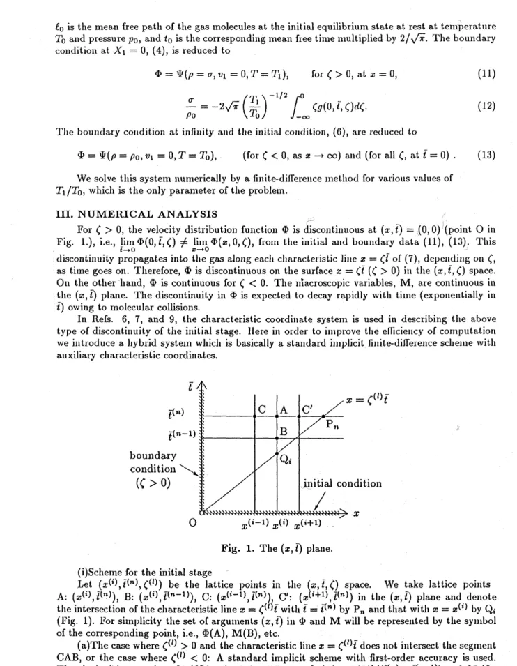
Fig. 1. The ($x,$$|\gamma$ plane.

(i)Schemefor the initialstage

Let $(x^{\langle i)},\overline{t}^{(n)}, \zeta^{(l)})$ be the lattice points in $tl\iota e(x,\overline{t})\zeta)$ space. We take lattice points

$A:(x^{(i)},\overline{t}^{(n)}),$ $B:(x^{(i)},\overline{t}^{(n-1)}),$ $C:(x^{(i-1)},\overline{t}^{(n)}),$ $C’:(x^{(t+1)},\overline{t}^{(n)})$ in the $(x,\overline{t})$ plane and denote

theintersectionof thecharacteristicline$x=\zeta^{(l)}\overline{t}$with$\overline{t}=\overline{t}^{(n)}$ by

$P_{n}$ and tbat witb $x=x^{(i)}$ by $Q_{i}$

(Fig. 1). For$si_{l}n$[)[_$icity$ theset of$\arg_{Ulne11}\iota_{S}(x,\overline{i})$in $\Phi$ and _$M$ will be represented by $t1_{1}e$symbol

of the corresponding point, i.e., $\Phi(A),$ $M(B)$, etc.

(a)The casewhere $\zeta^{(l)}>0$and the characteristic line$x=\zeta^{(l)}\overline{t}$doesnot intersect thesegment

CAB, or the case where $\zeta^{(1)}<0$: A standard implicit scheme with first-order accuracy is used.

235

$t^{\langle 1}T^{\mathfrak{n}^{\iota)}-1)}-\overline{t}\underline{C}_{x^{(i-1)(i)}}\ovalbox{\tt\small REJECT}\neq_{x^{\neg-\Phi^{+}(Q_{i})^{=\zeta^{(l)}\overline{t}}}}^{\overline{\triangle\overline{t}}}Q_{i}$

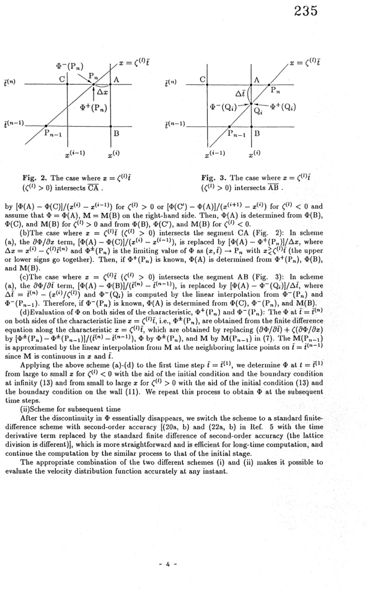
Fig. 2. The casewhere$x=\zeta^{(l)}\overline{t}$ Fig. 3. The case$wl\iota erex=\zeta^{(l)}\overline{t}$

$(\zeta^{(l)}>0)$intersects CA . $(\zeta^{(1)}>0)$ intersectsAB

.

by $[\Phi(A)-\Phi(C)]/(x^{(i)}-x^{(i-1)})$ _for $\zeta^{(t)}>0$ or $[\Phi(C’)-\Phi(A)]/(x^{(i+1)}-x^{(i)})$ for $\zeta^{(l)}<0$ and

assume that $\Phi=\Phi(A),$ $M=M(B)$on the right-hand side. Then, $\Phi(\Lambda)$ isdetermined from $\Phi(B)$, $\Phi(C)$, and $M(B)$ for $\zeta^{(l)}>0$ and from $\Phi(B),$ $\Phi(C’)$, and $M(B)$ for $\zeta^{(l)}<0$.

(b)Tbe case where $x=\zeta^{(l)}\overline{t}(((l)>0)$ intersects the segment $C\Lambda$ (Fig. 2): In scheme

(a), the $\partial\Phi/\partial x$ term, $[\Phi(A)-\Phi(C)]/(x^{(i)}-x^{(i-1)})$, is replaced by $[\Phi(A)-\Phi^{+}(P_{n})]/\Delta x$, where

$\Delta x=x^{(i)}-\zeta^{(.l)}\overline{t}^{(n)}$ and $\Phi^{\pm}(P_{n})$ is $tl\iota e$limiting value of$\Phi$ as (

$x,$$t_{l}^{arrow}arrow P_{n}$ with $x_{<}^{>}\zeta^{(1)}\overline{t}$(theupper

or lower signs go together). $T1_{1}en$, if$\Phi^{+}(P_{n})$ is known, $\Phi(A)$ is determined from $\Phi^{+}(P_{n}),$ $\Phi(B)$,

and$M(B)$.

(c)The case where $x=\zeta^{(l)}\overline{t}(\zeta^{(l)}>0)$ intersects the segment AB (Fig. 3): In scbeme

(a), the $\partial\Phi/\partial\overline{t}$ term, $[\Phi(\Lambda)-\Phi(B)]/(t^{T^{n)}}-\overline{t}^{(n-1)})$, is replaced by $[\Phi(\Lambda)-\Phi^{-}(Q_{i})]/\Delta\overline{t}$, where

$\Delta\overline{t}=\overline{t}^{(n)}-(x^{(\mathfrak{i})}/\zeta^{(1)})$ and $\Phi^{-}(Q_{j})$ is computed by the linear interpolation from $\Phi^{-}(P_{n})$ and

$\Phi^{-}(P_{n-1})$

.

Tberefore, if$\Phi^{-}(P_{n})$ is known, $\Phi(A)$ isdetermined fiom $\Phi(C),$ $\Phi^{-}(P,.))$

and

$M(B)$.

(d)Evaluationof$\Phi$onbothsidesoftbecharacteristic, $\Phi^{+}(P_{\iota})$ and$\Phi^{-}(I_{1}^{\supset})$: ’l’he$\Phi$ at$\overline{t}=\overline{t}^{(n)}$

on both sides of$t1_{1}e$characteristic line$x=\zeta^{(1)}\overline{t}$, i.e., $\Phi^{\pm}(P_{1})$, are obtained from$t1_{1}e$finitedifference

equation along $t1_{1}e$ characteristic $x=\zeta^{(l)}\overline{t}$, which are obtained by replaciIig $(\partial\Phi/\partial t\gamma+\zeta(\partial\Phi/\partial x)$ by $[\Phi^{\pm}(P_{n})-\Phi^{\pm}(P_{n-1})]/(\overline{t}^{(n)}-\overline{t}^{(n-1)}),$ $\Phi$ by $\Phi^{\pm}(P_{1})$, and $M$ by$M(P_{n-1})$ in (7). The$M(P_{r\cdot-1})$

is $approxin\iota ated$by tbelinear interpolation from$M$at tbe neigbboringlattice pointson$\overline{t}=\overline{t}^{(\iota-1)}$

since$M$ is continuous in $x$ and $\overline{t}$

.

Applying the above scheme $(a)-(d)$ to the first timestep $\overline{t}=\overline{t}^{(1)}$, we determine $\Phi$ at $t=\overline{t}^{(1)}$

from large to small $x$ for $\zeta^{(l)}<0$ with the aid of the initialcondition and the boundary condition

at infinity (13) and from small to large$x$ for$\zeta^{\langle t)}>0$ with the aid of tlie initial condition (13) and

the boundary condition on the wall (11). We repeat this process to obtain $\Phi$ at the subsequent

timesteps.

(ii)Scheme for subsequent time

Afterthe discontinuityin $\Phi$essentially disappears, we switch the scheme to astandard

finite-difference scheme with second-order accuracy [($20a$, b) and ($22a$, b) in lLef. 5 witb tbe time

derivative term replaced by the standard finite difference of second-order accuracy (tlie lattice

division isdifferent)], whicb ismorestraightforwardandis efficientforlong-time computation, and

continuethe computationby thesimilar process to tliat of the initial stage.

The appropriate combination of the two different schemes (i) and (ii) makes it possible to

236

IV. RESULT

Finally, wesummarize themain result of the numericalanalysis.

A. The caseofsudden heating $(T_{1}/T_{0}>1)$

We sbow the time development of $t1_{1}e$ profiles of the temperature $T$, pressure $p$, and flow

velocity $v_{1}$ for $T_{1}/T_{0}=2$ in Figs. $4a(0\leq t/t_{0}\leq 16),$ $4b(10\leq t/t_{0}\leq 100)$, and $4c(100\leq t/t_{0}\leq$

10000), where the scales of the ordinates, common to the tbree figures, are shown in Fig. $4a$

.

In

Table I,wegive the correspondingtimeevolutionoftlievalues oftbe energy flow$H_{1}$, normal stress $p_{11)}$ temperature$T$, and pressure$p$ at the wall, where$H$: is $t1_{1}e$energyflow vector $(H_{2}=H_{3}=0)$

and$p_{ij}$ is thestress tensor $(p_{12}=p_{13}=p_{23}=0)$ defined, respectively, by

$H_{i}= \frac{1}{2}\int\xi_{i}\xi_{j}^{2}fd\xi_{1}d\xi_{2}d\xi_{3}$, $p_{ij}= \int(\xi:-v_{i})(\xi_{j}-v_{j})fd\xi_{1}d\xi_{2}d\xi_{3}$. (14)

Thepressurerisenear$t1_{1}e$wall by sudden heating pushes$t1_{1}e$gasawayfrom the wall and sends

out a compression wave (shock wave) toward infinity in tbe gas. Then, $t1_{1}e$density near the wall

begins to decrease because there is no mass injection from the wall to compensate $t1_{1}e$ gas flow.

Thisleads to apressure decrease since theenergy $snpp_{-}Lyefrom$ tliewall, whichdecreaSes with the

temperature rise near the wall, is insu(ficient, and an expansion wave is sent out to $1111$} after the shock wave. The expansion wave finally overtakes the shock wave and weakensit. For large$t/t_{0}$,

the amplitude ofthe shock wave decreasesvery slowly, and its propagation speed approaches the sound speed at the equilibrium state at rest with temperature$2_{0}^{1}$ and ])_{$1^{\cdot}essurep_{0}$}

.

As

regards the

temperature field, only a small part of the disturbance propagatesas tlie sbock wave, and the rest

diffusesslowly. Thevelocity profilebehind theshock wavehas a shoulder. Theregion neartbe wall

where the slope of the profile is larger corresponds to $t1_{1}e$ diffusion region. The gas is heated by

diffUsion

andispushed outward there. The heatingand piston effect getsweakeras time goes on. Correspondingly, expansion waves are continuously sent out to accommodate tbedif[usion _region and the region behind the sbock wave. Thus, the region between the $sl\iota oulder$ and sbock wave

is the region of expansion waves. Since a wave sent out at later time is weaker, the variation of physical quantities in the expansion wave region is larger farther away from the wall, that is, the

variation is largest just behind theshock wave (see Fig. $4c$). In the limit of$t/t_{0}arrow\infty$, tliestate

ofthe gas approaches tlie uniform equilibrium state at rest with temperature$T_{1}$ and pressure$J^{l}o$

.

For$T_{1}/T_{0}=2$, the reduced velocity distribution function$g$ at $t/t_{0}=0.5,2$, and

10

is sbown

in

Fig.

5

asafunction of$(2RT_{0})^{-1/2}\xi_{1}$

.

The discontinuity of_$g$ in the

gas

attenuatesrapidly with

time due tomolecularcollisionsandis invisible at $t/t_{0}=10$

.

The discontinuity at $tl\iota e$ wall decays

slowly.

In Fig. 6 and Table I, we give some results for asmall temperature rise, i.e., $T_{1}/T_{0}=1.1$

.

$T1\iota e$feature of the flow field is very similar to that for $T_{1}/T_{0}=2$except that the amplitude of the

disturbanceissmall*. In TableI, the analytical

resnlts1

of$t1_{1}e$ temperature and pressure forshort

time and long time based on $t1_{1}e$linearized equation, suppleniented by more recent and accurate

$data^{1}$ for the numerical coeflicients, arealso $sl_{1}o\backslash VI1$ forcomparison.

B. The case of sudden cooling $(T_{1}/T_{0}<1)$

For$T_{1}/T_{0}=0.5$, we show $tl\iota e$ timedevelopment of tbe profiles of_{$T,$ $p$}, and $v_{1}i_{l1}$ Figs. $7a,$ $b,$ $c$

and the time evolution ofthe values of $H_{1},$ $p_{11},$ $T$, and $p$ at $t1_{1}e$wall in Table II. In contrast to

the case of $1_{1}eating$₎ sudden cooling gives rise to a pressure decrease near the wall, $w1_{1}ic1_{1}$ causes

a

gas

flow toward the wall and sends out anexpansion wave. Owing to the

gas

flow, the density

near the wall begins to

increase.

This leads to the pressure rise, and a compression wave is sent

out. The compression wave overtakes the preceding expansion wave and weakens it. Only a small part ofthe disturbance in thetemperaturepropagates as tlie expansion wave, and$t1_{1}e$rest diIfuses

slowly. In Fig. 8, weshow$t1_{1}e$reduced velocity distribution function_$g$ at$t/t_{0}=0.5,2$, and

10

for $T_{1}/T_{0}=0.5$

.

$T1_{1}e$ results for a small temperature drop, i.e.,$T_{1}/q_{0}^{1}=0.9$, are shown in Fig. 9 and Table II,

wheresomeresults of thelinearized

analysis1

arealso given. Tbe pattern of thetimedevelopment

ofthe disturbance

is

very similar tothat for $T_{1}/T_{0}=0.5$

.

237

The lattice system used in the computation is as follows ($t1_{1}e$ dimensionless variables $x,\overline{t},$ $\zeta$

are used below). Tbe molecular velocity $\zeta$is limitcd to I.be finiteint,$CI^{\cdot}V:\iota 1-Z\leq\zeta\leq 7_{J}$ wit.h $Z=6$ $(?_{1}^{1}/2_{O}^{\tau}<1)$ or 7 $(’l_{1}^{1}/2_{0}^{\tau}>1)$, wbich is divided into 120 nonunifounsections with tbe $111i_{Il}imu\iota n$

width $2.68x10^{-2}\sim 3.07x10^{-2}$ _around $\zeta=0$ and the maximum width 0.305 $\sim 0.373$ around $\zeta=\pm Z$

.

The space coordinate$x$ is limited to the finite interval $0\leq x\leq D$, where tbe subregion $0\leq x\leq D_{1}(D_{1}\cong 21)$ is divided into $N_{1}$ nonuniform sections $\backslash vitl\iota$ tbe $111i_{1}\iota i_{111}u1l1$ widtb $\triangle,,\iota$

around $x=0$ and the maximum width $\Delta_{M}$ around _{$x=D_{1}$}, and the rest $D_{1}\leq x\cdot\leq D$ is divided

into $N_{2}$ uniformsections with the width $\Delta_{M}$

.

For$0\leq\overline{t}\leq 100,$ $D\cong 21\sim 133,$ $N_{1}=1500\sim 375$, $N_{2}=0\sim 1125,$ $\Delta_{m}=0.0025\sim 0.01$, and $\Delta_{\Lambda I}=0.025\sim 0.1$; for $100<\overline{t}\leq 2000,$ $D\cong 283\sim$

2383, $N_{1}=188\sim 24,$ $N_{2}=1312\sim 1476,$ $\Delta_{n}=0.02\sim 0.16$, and $\Delta_{\Lambda f}=0.2\sim 1.6$; and for

$2000<\overline{t}\leq 10000,$ $D\cong 15983,$ $N_{1}=24,$ $N_{2}=9976,$ $\Delta_{m}=0.16$, and $\Delta_{M}=1.6$. The time step

in$\overline{t}$is

changed, according as time, from tbe minimum step 0.0025 $(0\leq\overline{t}\leq 100)$ to tlte maximum

step 0.1 $(2000<\overline{t}\leq 10000)$

.

Let us denote the lattice system described above by $L1$

.

For an accuracy test, we prepared

two coarser lattice systems $L2$ and $L3$, i.e., $L1$ with double the tirne step intervals $(L2)$ and $L1$

with double the space lattice intervals $(L_{\backslash }!))$ and carried out tbe colllpnlalioll until $\overline{t}=100$. To

showthe data, we introduce

$S(x,\overline{t})=1nax(|M(L1)-M(L2)|, |M(L1)-M(L3)|)$,

(for eachlattice point in $(x,\overline{t})$ commonto $L1,L2,andL3$),

$\overline{S}(t\gamma=0\max_{\leq x<\infty}S(x,\overline{t})$,

$w1_{1}ereM$ represents the macroscopic variables $T_{o}^{-1}T,$ $p_{0}^{-1}p$, etc. and $\Lambda\cdot f(L1)$, etc. indicate $tl\iota eM$

computed on the basis of lattice $L1$, etc. $TheIl,$ $S(O,$$t\gamma$ for$p_{0}^{-1}(21l’1_{0}^{1})^{-1/2}lI_{1},$ $p_{0}^{-1}p_{11},2_{0}^{\tau-1}T$, and $p_{0}^{-1}p$ are, respectively, less $t1_{1}an$ thefollowing (cf. $r_{1^{\urcorner}ables}$Iand II):

$3.0x10^{-4},1.8x10^{-4},3.7x10^{-4}$_{, and} $3.2x10^{-4},$ $(T_{1}/T_{O}=2)$, $3.1x10^{-S},$ $1.4x10^{-s},$ $3.0x10^{-s}$, and $1.7x10^{-s},$ $(T_{1}/T_{0}=1.1)$, $4.0x10^{-4},1.4x10^{-4},3.0x10^{-4}$, and $1.9x10^{-4},$ $(T_{1}/T_{0}=0.5)$,

$0.1\leq\overline{t}\leq 100$

.

$3.2x10^{-s},\cdot 1.5x10^{-s},$ $3.0x10^{-5}$, and $1.9x10^{-s},$ $(T_{1}/T_{0}=0.9)$,

$\overline{S}(10n)(m=1,2, \cdots , 10)$ for $T_{o}^{-1}T,$ $p_{0}^{1}p$, and $(21l\mathcal{I}_{\acute{0}})^{-1/2}v_{1}$ are, respectively, less $t1\iota_{\dot{C}}\iota I1$ the fol-lowing: $1.4x10^{-3},2.0x10^{-3}$, and $9.9x10^{-4},$ $(T_{1}/T_{0}=2)$, $5.9x10^{-S},$ $1.1x10^{-4}$, and $6.1x10^{-s},$ $(T_{1}/T_{O}=1.1)$, $9.0x10^{-4},8.8x10^{-4}$, _and $5.2x10^{-4},$ $(T_{1}/T_{0}=0.5)$, $5.8x10^{-5},1.1\cross 10^{-4}$, and $6.1x10^{-5},$ $(T_{1}/T_{0}=0.9)$. REFERENCES

1. Y. Sone, J. Phys. Soc. Jpn. 20, 222 (1965).

2. A. A. Kovitz and K. 1I. lIellman, in Rarefied $G$as Dynamics, edited by D. Dini

(Editrice$rr_{ecnico}$ Scientifica, Pisa, 1971), p. 811.

3. Y. Sone, K. Aoki, and I. Yamashita, in Rarefied

Gas

Dynamics, edited by V. C. Boffi and

C. Cercignani (Teubner, Stuttgart, 1986), Vol. 2, p. 323.

4. Y. Soneand $1I$

.

Sugimoto, J. Vac. Soc. Jpn. 31, 420 (1988) (in Japanese).

5. $I${. Aoki, Y. Sone, and T. Yamada, Phys. Fluids A (to be

published).

6. H. Sugimoto and Y. Sone, J. Vac. Soc. Jpn. 32, 214 (1989) (in Japanese).

7. Y. Sone and II. Sugimoto, inAdiabatic Waves in Liquid-Vapor $Systelns$,

edited by G. E. A. Meier and P. $\Lambda$

.

_{$T1_{1O111}p_{SO11}$}

(Springer, Berlin, 1990), p. 293.

8. C. It. $C1_{1t1},$ $Pl\iota ys$. Fluids 8, 12 (1965).

9. II. Sugimoto, master’s thesis, Kyoto University (1989) (in Japanese).

238

$tD\frac{1}{\overline{r}}$ そ $\succ,$ $oi$ $\frac{r}{\cup}$ $||$ $\underline{o}$ 膚 $\succ v\backslash$ つ $\xi_{\neg}^{\sim}$ $\omega$ $\sim$ $\circ$ $O$ $\not\supset\infty$ て $0_{1}$ 臼 $g$ $Q)$ .$\underline{O}$ $A\infty$ $\in\dashv$ $-v$

.

轟 $1\circ$ $\overline{O}$ ぽ$\overline{r}$ $.-$ $\approx$ $h.\circ$ 6 $-\wedge$ $o$ $||$ $arrow$ 曽

.

百$\circ i^{\wedge}$ 科 $\overline{||}$ 歌王 $’\circ$ 何 $\circ\not\in$ $Q_{\backslash }^{\wedge}rightarrow$ ト $||\circ$ $b_{\circ}\backslash rightarrow$ $\underline{\omega^{0}\{}r^{\overline{\circ}-}$ $\not\in_{O}-\mu\circ_{\wedge}\wedge$ $b-$ $O_{t}\infty$ . $A^{Q)}arrow$ $N^{\wedge}$ $-$ $\bigvee_{\circ}N_{\wedge}^{\wedge}\overline{||}$ $\inftyrightarrow$ $\overline{\omega}$ $||$ $\underline{\S}$ $\propto 8\underline{g}g\circ$ $\frac{O}{Q),\succ}\circ\backslash \S$ 呂 て $-\wedge-O^{\wedge}$

.

$\underline{gQ)}\dot{\circ}\Omega\underline{\circ\circ}$ $R^{(])}\infty(\supset^{\wedge}\infty i.\underline{\circ^{\wedge}\circ}$ $\xi\dashv$ $||$ $||$ $\triangleleft$ $\infty^{O}\infty^{O}$ $\backslash \backslash$ $bO–$ 角$\underline{\circ}3$

240

$’ \frac{\infty t!1}{\circ}\dot{\Omega}=^{t}$ $\underline{r}\wedge^{o_{||}}$ $\underline{o}$ 虞 $\succ Q)\backslash$ $o^{\tilde{h_{o}}}\omega$

.

$\not\supset\cdot\mapsto$ $\tau\circ$, 臼 $e$ $\simeq\omega.\frac{\circ}{arrow}$ $\in\dashv\underline{U}$

.

$\underline{\approx}$ . 召 $r^{\overline{\frac{o}{}}} \frac{r}{\circ}$ $\dot{\Omega}$

.

$O\overline{\circ}$ $||$ $rightarrow$ 虞

.

百$N^{\wedge}$ 科 $\overline{||}^{\wedge}$ ダ王 $’ \frac{\circ}{‘ 6}\circ s$ へ $rightarrow$ $11$ ト $0$ $4_{\circ^{4}}\backslash \infty$ のへ $\underline{Q)}r\circ-$ $*_{O}-\iota\circ_{\wedge}\wedge$ $h-$ $\approx\infty$

.

$\neq^{\omega}arrow$

.

$\infty^{\wedge}$ $\overline{O}N^{\wedge}\overline{||}$ $arrow\overline{Qj}\overline{||}^{\wedge}\underline{S}$ $\alpha 8\underline{g}g\circ$ $\frac{O}{\Phi}$ $\not\in$ 呂 $\succ\theta tO1$ て $-\wedge\circ^{\wedge}$ .目 $\hat{\dot{o}}^{3}u\underline{\circ\circ}$ $rightarrow B\Phi\dot{\circ}^{\wedge}\infty\circ^{\wedge}\sim\circ$ $\xi\dashv$ $||$ $I|$ $\iotaarrow$ $\sim^{O}\sim^{O}$ $\backslash \backslash$ $bD–$ $\dot{\overline{Q}}\underline{6}\underline{\cup}$