INSTABILITY OF THE MOTION OF AN IDEAL FLUID CONTAINED IN 2-SPHERE AS A GEODESIC EQUATION

INSTABILITY OF THE MOTION OF AN IDEAL FLUID

CONTAINED IN 2-SPHERE AS A GEODESIC EQUATION

KYO YOSHIDA $(_{-}^{\pm}\mathrm{f}\mathrm{f}\mathrm{l} ae_{\mathrm{J}\backslash })$

ABSTRACT. The Euler’s equationforan incompressiblefluid filled in aRiemannian

manifold $D$ is regarded as a geodesic equation on thegroup ofvolume-preserving

diffeomorphisms of$D$ provided with a one-sided invariant metric. A negative

sec-tional curvature impliesinstability of thegeodesic with respecttothecorresponding

flow and perturbation. The exponential growth ofthe perturbation is estimated

from the values of the sectional curvatures.

The expression ofthe components ofRiemanniancurvature tensor ofthe group

of area-preservingdiffeomorphismson2-sphereisgiven in explicit formulas through

$3-j$ coefficients.

The meansectionalcurvature associated with the flow describedbythe flow

func-tion$Y_{2}^{0}$isestimated for example and the resultsuggeststhat the initial perturbation

$\epsilon$ grows to

$3\cross 10^{2}\epsilon$ after the period during which the particles on $u=cos \theta=\frac{1}{2}$

rotate around $z$-axis.

1. INTRODUCTION

Let $T(t)$ be the map which maps the configuration of some fluid particles at the time $t_{0}$ to the configuration at the time $t$. Then the motion of the fluid is regarded

as this time dependent map $T(t)$. Continuity of the fluid requires this map $T(t)$ to be diffeomorphism. We will regard the diffeomorphism $T(t)$ as a point element in the

group of the diffeomorphisms. From now on, $T(i)$ will be denoted by $x_{t}$.

The Euler’s equation for an ideal incompressible fluid filled in a Riemannian man-ifold $D$ is regarded as a geodesic equation on the group of volume-preserving

dif-feomorphisms of $D$ provided with a one-sided invariant metric [2]. Let the group

be denoted by $\mathfrak{D}_{vol}(D)$. The geodesic $x_{t}\in \mathfrak{D}_{vo}\iota(D),$ $t\in \mathrm{R}$, satisfies the following geodesic equation:

(1.1) $\nabla_{\dot{x}_{t}}\dot{x}_{t}=0$,

where $\dot{x}_{t}=\frac{d}{dl}x_{t}\in T_{x_{t}}\mathfrak{D}_{vol()}D$, $x_{t}\in \mathfrak{D}_{vol}(D)$. The metric $g$, the Riemannian connection

$\nabla$, the Riemannian curvature tensor $R$

a vector field along the geodesic $x_{t}$ which satisfies the following Jacobi equation:

(1.2) $\nabla_{\dot{x}_{t}}^{2}Y+R(Y,\dot{x}_{t})\dot{x}_{t}=0$.

A Jacobi field is an infinitesimal variation of the geodesic $x_{t}$ and is uniquely

deter-mined by the values of $Y$ and $\nabla_{\dot{x}_{a}}Y$ at one point $x_{a}$ (or an initial point $x_{0}$) on the

geodesic. We obtain from (1.2) the following equation:

(1.3) $\frac{d^{2}}{dt^{2}}||Y||^{2}=2(||\nabla_{\dot{x}_{t}}Y||2-g(R(Y,\dot{X}_{t})\dot{X}t,$_$Y))$.

The length $||Y||$ of the Jacobi field $Y$ grows exponentially with respect to $t$ if the

value of the sectional curvature $\kappa(Y,\dot{x}_{t})$ is negative. For a geodesic $x_{t}$ parameterized

to satisfy the property $||\dot{x}_{t}||=1$ for all $t$, the minimum exponent of the exponential

growth with respect to$t$for the fixed value of$Y$at one point$x_{a}$ isgiven by$\sqrt{-\kappa(Y,x_{a})}$

and this is the case when $\nabla_{\dot{x}_{a}}Y=0$. If we regard the values of $Y$ and $\nabla_{\dot{x}_{t}}Y$ at $x_{0}$ as

initial perturbations, the negative sectional curvature implies the instability of the

geodesic. This instability suggests that it is $\mathrm{i}\mathrm{m}$

. possible to predict the passive scalar

advected by the motion of the ideal incompressible fluid over a certain period, and the period is estimated from the value of the sectional curvature $\kappa$.

The flow over $2- \mathrm{s}_{\mathrm{P}^{\mathrm{h}\mathrm{e}\mathrm{r}\mathrm{e}}}(s^{2})$ may be regarded as a simplified model of the motion

of atmosphere over the earth.

2. BASIC NOTATIONS

Let $S^{2}$ be defined in $\mathrm{R}^{3}$ by the equation $x^{2}+y^{2}+z^{2}=r^{2}$ and its Riemannian

metric $(, )$ be defined as the restriction of the standard Euclidean metric of$\mathrm{R}^{3}$

.

Let $(\theta,\varphi)$ and $(u, \varphi)$ be coordinates defined by:

$x=r\sin\theta\cos\varphi$

(2.1) $y=r\sin\theta\sin\varphi$

$z=r\cos\theta=ru$.

and the Riemannian metric in $S^{2}$ _{$( , )$} has components $( \frac{\partial}{\partial u}, \frac{\partial}{\partial u})=\frac{r^{2}}{1-u^{2}}$

(2.2) $( \frac{\partial}{\partial\varphi}, \frac{\partial}{\partial\varphi})=r^{2}(1-u^{2})$

$( \frac{\partial}{\partial u}, \frac{\partial}{\partial\varphi})=0$

.

The Riemannian volume (area) element $\mu$ is given by:

where $S=4\pi r^{2}$ is the area ofthe sphere.

Let the group

_of

volume-preserving diffeomorphisms$\mathfrak{D}_{vol}(S^{2})$

of

$S^{2}$ acts on$S^{2}$ from

right. The elements of$T\mathfrak{D}_{vol()}s^{2}$ induce vector fields on $S^{2}$ with divergence-free. The

set of vector fields on $S^{2}$ with divergence-free will be denoted by _{$X_{vol}(s2)$}, and the

vector field induced by $A\in T\mathfrak{D}_{vol}(s2)$ will be denoted by $A^{*}$

.

The Riemannian

metric $g$ on $\mathfrak{D}_{vol}(s^{2})$ is induced from the metric $(, )$ on $S^{2}$ as follows:

(2.4) $g_{a}(A, B)= \int_{S^{2}}(A^{*}, B^{*})\mu$, $a\in \mathfrak{D}_{vol}(s^{2}),$$A,$$B\in T_{a}\mathfrak{D}_{vol}(S^{2})$

.

This

_m.e.tric

is

_{left-invariant.}

Remark. In [2] ,$[3],$ $\mathfrak{D}_{vol}(D)$ is (implicitly) determinedto act on $D$ from left, so that

the corresponding metric is right-invariant. For $X\in X_{vol}(s^{2})$, we have:

(2.5) $0=,$ $divX=L_{X}\mu=d\iota_{X}\mu$,

where $L_{x}$ is the Lie derivative with respect to the vector field $X$ and $\iota_{X}$ is the

contraction with $X$ defined as follows:

(2.6) $\iota x\mu(Y)=\mu(X, Y)$.

(2.5) is obtained from the identity $L_{X}=d\mathrm{o}\iota_{X}+\iota_{X}\mathrm{o}d$. Since de Rham cohomology group $H^{1}(S^{2})$ is $0$, there exists a unique function $\psi x$ on $S^{2}$ for each _{$X\in X_{vol}(S2)$}

satisfying:

(2.7) $d\psi_{\mathrm{x}=\iota_{X}}\mu$.

$\psi_{X}$is said to be a

fiow function

ofthevector field$X$ on $S^{2}$

.

Let $X_{\psi}$ denote the vector

field whose flow function is $\psi$. $X_{\psi}$ is expressed in the coordinate $(u, \varphi)$ by

(2.8) $X_{\psi}= \frac{4\pi}{S}(\frac{\partial\psi}{\partial u}\frac{\partial}{\partial\varphi}-\frac{\partial\psi}{\partial\varphi}\frac{\partial}{\partial u})$ .

$X\psi$ is a Hamiltonian vector field of the function $\psi$’ with respect to the symplectic

2-form $\mu$. The

$\acute{b}$

racket product $\{$ , $\}$ of two functions $f$ and $g$ on $S^{2}$ is defined by: (2.9) $\{f,g\}=-\mu(xf,\mathit{9}X)$.

Note that our definition of the bracket differs in sign from the conventional definition of the Poisson bracket. Let $A$ and $B$ be the elements of the Lie algebra$0_{vol}(S^{2})$ (.i.e.

a set of left invariant vector fields) of the group $\mathfrak{D}_{vol}(s2)$ and $e$ denote the identity

$X_{vol}(S^{2})$ and the mapping $X\in X_{vol}(s^{2})arrow\psi_{X}\in C^{\infty}(S^{2})$ are both isomorphisms

with respect to each corresponding bracket, namely:

(2.10) $[A_{e}^{*}, B_{e}^{*}]=[A, B]_{e}*$, $A,$$B\in v_{vol}(s^{2})$,

(2.11) $\{\psi_{x}, \psi_{Y}\}=\psi_{[}X,Y]$, $X,$ $Y\in X_{vo}\iota(S2)$.

Consequently, we obtain:

(2.12) $\{\psi_{A_{\mathrm{e}}}*, \psi B^{*}\mathrm{e}\}=\psi_{[A,B]_{e}}*$,

and from nowon, we identify the function $\psi_{A_{\mathrm{e}}*}$ on $S^{2}$ with the element $A$of the Lie

algebra $0_{vol}(S^{2})$. The bracket product $\{$, $\}$ of two functions on $S^{2}$ is also identified

with the Lie bracket of the Lie algebra $0_{vol}(S^{2})$. We formally complexify the Lie

algebra $0_{vol}(s2)$ and the above identification enable to express the elements of the

algebra $\emptyset_{vol}(S^{2})$ by the linear combinations of the spherical harmonics $Y_{l}^{m}$. The

orthonormal basis with respect to the metric $g$ will be denoted by $\tilde{Y}_{l}^{m}$: (2.13)

(2.14) : $g_{e}(Y_{l^{\prime ib}}, \mathrm{Y}_{l^{-}\mathrm{I}=}\prime\prime\prime u(-\perp)’\prime v_{\delta\prime}ll\delta mm’\cdot$

Let $C$ denote the structure constants, namely:

(2.15) $\{\tilde{Y}_{l_{1}}^{m_{2}},\tilde{Y}_{l_{2}}^{m}2\}=\sum_{lm}C\tilde{Y}_{l}^{m}$.

We now consider the Riemannian connection $\nabla$ associated with the Riemannian

metric $g$. Let $X(M)$ denote the set of vector fields on M. $\nabla xY\in X(\mathfrak{D}_{vo}l(S^{2}))$, the covariant derivative of $Y$ in the direction of $X$, is a bilinear function of _{$x_{\iota},Y\in$}

$X(\mathfrak{D}_{vol}(s2))$. $\nabla$ is uniquely defined to satisfy the following conditions:

(2.16) $\nabla_{X}Y-\nabla_{Y}x-[X, Y]=0$,

(2.17) $X(g(Y, Z))=g(\nabla_{X}Y, z)+g(Y, \nabla_{X}z)$.

for any $X,$$Y,$ $Z\in X(\mathfrak{D}_{vol(}s2))$. For $X,$$Y,$$Z\in\eta_{vol}(s2)$, we obtain the following

formula from (2.16) and (2.17).

$i^{:}$

.

(2.18) $g( \nabla x^{Y}, z)=\frac{1}{2}(g([X, Y], z)+g([z, x], Y)+g([Z, Y],X))$.

. $\backslash \cdot$

. .:

The

_{Christoffel’s}

symbols $\Gamma$ is defined by:

$.\mathrm{t}$

..

$l\backslash$.

From $(2.18),(2.14)$ and (2.19), weobtain the following formula:

(2.20) $\mathrm{F}$

$= \frac{1}{2}(C+(-1)^{m_{1}}C+(-1)^{m_{2}}C)$

.

The Riemannian curvature

_{transformation}

$R$ associates to each pair of vector fields

$X$ and $Y$ the linear transformation:

(2.21) $R(X, Y)=\nabla x\nabla_{Y}-\nabla Y\nabla_{X}-\nabla_{[Y}X,]$

.

The Riemannian curvature tensor, also denoted by $R$, is defined by:

(2.22) $R(X_{1,2,\mathrm{s}}XX, X_{4})=g(R(x_{3}, X4)X_{2},$$X_{1})$, where $X_{1},$

$\ldots,$$X_{4}$ are vector fields. The Riemannian curvature tensor $R$ satisfies the

following properties:

$R(X_{1}, X_{2}, x3, X_{4})=-R(X_{2}, X_{1,3}X, x_{4})$, (2.23) $R(X_{1}, X_{2}, x3, X_{4})=-R(X_{1}, x_{2}, x4, x_{3})$,

$R(X_{1}, X_{2,\mathrm{s},X_{4}}X)+R(x_{1}, x_{3}, X_{4}, X_{2})+R(X_{1}, X_{4}, x2, X_{3})=0$.

If$X_{1}$ and $X_{2}$ are orthonormal, the value:

(2.24) $\kappa(X_{1}, X_{2})=R(X_{1}, X_{2}, x1, X_{2})$

is called the sectional curvature of the 2-dimensional plane containing the directions

of $X_{1}$ and $X_{2}$

.

If $X_{1}$ and $X_{2}$ are not orthonormal, then the corresponding sectional

curvature is given by:

(2.25) $\kappa(X_{1},X_{2})=\frac{R(X_{1},X_{2},x1X_{2})}{g(X_{1},X_{1})g(x_{2},X_{2})-(g(X_{1},x2))2},$.

We employ the following abbreviations:

(2.26) $R=R(\tilde{Y}_{l_{1}’\iota_{2}’ l}^{m_{1}}\tilde{Y}m2\tilde{Y}m_{3},\tilde{Y}_{l}m_{4})34$ ’

3. DISCUSSIONS

The explicit formulas of the Riemannian curvature tensor $R$ and the sectional

curvature $\kappa$ are obtained in [14]. They are expressed through $3-j$

coefficients.

The

$3-j$ coefficients

can be computed from the following formula [13].

Here is the theorem for the explicit formulas of the Riemannian curvature tensor

$R$ and the sectional curvature $\kappa$.

Theorem 3.1 (Yoshida [14]).

_If

$l_{1}+l_{2}+t$ is $odd_{f}$ the structure constants are ex-pressed by:

otherwise

Corollary 3.1. With the structure $conStant_{\mathit{8}}C$, the

Christoffel’s

symbols $\Gamma$ and the

Riemannian curvature tensor $R$ are given by the

formulas:

(3.4) $\Gamma=\frac{1}{2\lambda}(\lambda-\lambda_{1}+\lambda_{2})c$ , (3.5)

$R=(-1)^{m_{1}} \sum_{lm}(\Gamma\Gamma$

$-\Gamma\Gamma$

$-C\Gamma)$

.

By virtue of this theorem, it is possible to compute the sectional curvature of any particular 2-dimensional plane in $T_{\mathrm{e}}\mathfrak{D}_{v\circ l(}S^{2}$). We are going to study the stability of

the azimuthal flow with the flow function $\hat{Y}_{l}^{0}$. We restrict the perturbations to the

flows described by the flow function $R_{a}^{*}\hat{Y}_{l}^{0},$

$,$ $a\in SU(2)$, where

$R_{a}^{*}$ is a pull back of

the function associated with the right action of $a$ on $S^{2}[14]$ We define the mean sectional curvature $\kappa_{m}(l, l’)$ associated with $l,$ $l’$ by:

$\kappa_{m}(l, l’)=\frac{1}{\Omega}\int_{SU(2})\kappa(\hat{Y}_{l}0, R_{a}*\hat{Y}_{l}^{0}, )da$ (3.6)

$= \frac{1}{2l’+1}\sum_{m}\hat{\kappa}$ ,

where $da$ is the Haal measure of $SU(2)$ and $\Omega$ is the measure of the whole group

defined to be $\int_{SU(2)}da$.

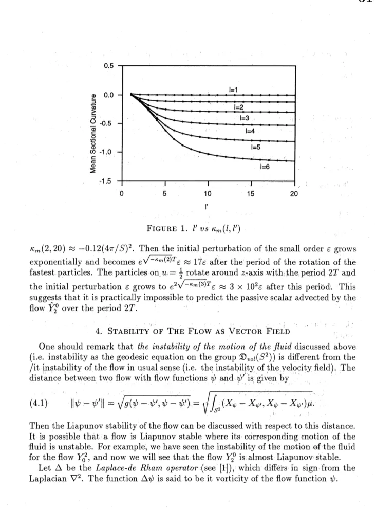
Fixing $r$ to be 1, actual computations of the mean sectional curvatures $\kappa_{m}(l, l’)$ are performed for some $l$ and $l’$, and the results are shown in Figure 1. Lukatskii [9] showed that $\lim_{larrow\infty^{\hat{\kappa}}(\begin{array}{l}l20\pm l\end{array})}=-(15/8\pi)\approx-0.60$. Since $\hat{\kappa}\approx-0.54\approx$

$0.90 \lim_{larrow\infty^{\hat{\kappa}}(\begin{array}{l}2l0l\end{array})}$ , we may consider $l=20$ is a sufficiently large value and reflects

some behavior when $l$ tends to be infinity.

Now we look at the flow $\hat{Y}_{2}^{0}$. The corresponding vector field

$X_{\hat{Y}_{2}^{0}}$ is given by:

(3.7) $X_{\hat{Y}_{2}^{0}}= \frac{1}{S}\sqrt{30\pi}u\frac{\partial}{\partial\varphi}$

.

The particles near the poles $u=\pm 1$ _{rotates around} $z$-axis faster and the

infe-rior limit of the period $T$ during which the particle rotates around $z$-axis is equal

$\cup$ $0$ $1\cup$ $\mathrm{i}3$

$|$’

FIGURE 1. $l’vS\kappa_{m}(l, l’)$

$\kappa_{m}(2,20)\approx-0.12(4\pi/S)^{2}$. Then the initial perturbation of the small order $\epsilon$ grows

exponentially and becomes $e^{\sqrt{-\kappa_{m}(2)}T}\epsilon\approx 17\epsilon$

after the period ofthe rotation of the fastest particles. The particles on $u \xi=\frac{1}{2}$ rotate around $z$,-axis with the period $2T$ and

the initial perturbation $\epsilon$ grows to

$e^{2\sqrt{-\kappa_{m}(3)}T}\epsilon\approx 3\cross 10^{2}\epsilon$

after this period. This

suggests that it is practically impossible to predict the passive scalar advected by the flow $\hat{\mathrm{Y}}_{2}^{0}$

over the period $2T$.

4.

STABILITYgOF

THE FLOW As VECTOR $\mathrm{F}\mathrm{I}\mathrm{E}\mathrm{L}’ \mathrm{D}$

$*\cdot$ \dagger. $l$. $.\cdot$ $\}$

.

. $t$.

One should remark that the instability

_of

the motion

_of

the

_fiuid

discussed above (i.e. instability as the geodesic equation on the group $\mathfrak{D}_{vol}(S2)$) is different from the

$/\mathrm{i}\mathrm{t}$ instability of the flowin usual sense (i.e. the instability of the velocityfield). The

distance between two flow with flowfunctions $\psi$ and $\psi’$ is given by

(4.1)

Then the Liapunov stability of the flow can be discussed with respect to this distance. It is possible that a flow is Liapunov stable where its corresponding motion of the fluid is unstable. For example, we have seen the instability of the motionof the fluid for the flow $Y_{0}^{2}$, and now we will see that the flow $Y_{2}^{0}$ is almost Liapunov stable.

Let $\triangle$ be the Laplace-de Rham operator (see [1]), which differs in sign from the

Lemma 4.1. $\mathrm{Y}_{l}^{0}$ is a stationary

flow.

Let $\phi_{0}$ be the initial perturbation and $Y_{l}^{0}+\psi_{t}$ satisfy the Euler’s equation. Then the following value conserves (is independent

_of

time $t$).

(4.2) $\frac{1}{l(l+1)}\int_{S^{2}}(\Delta\phi_{t})^{2}\mu-||\phi t||2$

Proof.

This is proved from the fact that the energy $( \frac{1}{2}||\psi_{t}||^{2})$ and the enstrophy $( \frac{1}{2}\int_{S^{2}}(\triangle\psi t)^{2})$ conserves for the solution of the Euler’s equation $\psi_{t}$ and that $\triangle Y_{l}^{0}=$

$l(l+1)Y_{l}^{0}$ (see [3]). $\square$

It is easy to see from Lemma 4.1 that flow $Y_{2}^{0}$ is almost Liapunov stable in the

following sense.

Theorem 4.1. Fix some arbitrary $\epsilon>0$. For $\phi_{t}$

defined

$ab_{ov}e$, the following

equa-tion:

(4.3) $|| \phi_{t}||^{2}\leq\frac{1}{\epsilon}(\int_{S}2)\frac{1}{6}(\triangle\phi 0)2\mu-||\phi t||^{2}$

holds

_if

(4.4) $I_{S^{2}} \frac{1}{6}(\triangle\phi_{t})2\mu\geq(1+\epsilon)||\phi_{t}||^{2}$ .

Remark. Since any flow not containing $Y_{1}^{m}$ (the rigid body motion mode) satisfies

the equation:

(4.5) $\int_{S^{2}}\frac{1}{6}(\triangle\phi_{t})^{2}\mu\geq||\phi_{t}||^{2}$,

the condition in Theorem 4.1 may almost be satisfied, choosing $\epsilon$ to be sufficiently

small.

5. SUMMARY

(1) The structure constants $C$ of the Lie algebra $\Phi_{vol}(s^{2})$ of the group of area-preserving diffeomorphism (motions of fluid) $\mathfrak{D}_{vol}(S^{2})$ of $S^{2}$ are obtained in

Theorem 3.1. They are expressed through $3-j$ coefficients. The components of the curvature tensorof the group $\mathfrak{D}_{vol}(S^{2})$ are expressed with the structure

constants. [14]

(2) The mean sectional curvature associated with $Y_{2}^{0}$ is computed and it is

esti-mated that the initial perturbation $\epsilon$grows to $3\cross 10^{2}\epsilon$ after the period during

which the particles on $u= \frac{1}{2}$ rotate around $z-\mathrm{a}\mathrm{x}\mathrm{i}_{\mathrm{S}},\mathrm{i}.\mathrm{e}.,\mathrm{t}\mathrm{h}\mathrm{e}$corresponding

(3) In spite of the instability of the motion of the fluid noted above for the flow

$\hat{Y}_{2}^{0}$, the flow $\hat{Y}_{2}^{0}$ is almost Liapunov stable as a vector field.

REFERENCES

1. Abraham,R. and Marsden,J.E $(‘ \mathrm{F}\mathrm{o}\mathrm{u}\mathrm{n}\mathrm{d}\mathrm{a}\mathrm{t}\mathrm{i}_{0}\mathrm{n}\mathrm{s}$of Mechanics”,Chapter 2. $\mathrm{B}\mathrm{e}\mathrm{n}\mathrm{i}\mathrm{a}\mathrm{m}\mathrm{i}\mathrm{n}/\mathrm{C}\mathrm{u}\mathrm{m}\mathrm{m}\mathrm{i}\mathrm{n}\mathrm{g}\mathrm{s}$,

1978.

2. $\mathrm{A}\mathrm{r}\mathrm{n}\mathrm{o}1^{\backslash }\mathrm{d},\mathrm{V}.\mathrm{I}$. $\mathrm{S}\mathrm{u}\dot{\mathrm{r}}$

la g\’eometrie diff\’entielle des de Lie de dimension infinie et ses application \‘a

l’hyrodynamique des fluides parfais, Ann.Inst. Fourier 16,no.l (1966), 319-361.

3. Arnold,V.I. ($‘ \mathrm{M}\mathrm{a}\mathrm{t}\mathrm{h}\mathrm{e}\mathrm{m}\mathrm{a}\mathrm{t}\mathrm{i}_{\mathrm{C}\mathrm{a}}1$MethodsofClassicalMechanics”,Appendix 2. Springer Verlag, New

York, 1978.

4. Arnold,V.I. and

_Khesin.

_’B.A.

$\mathrm{T}_{0}\mathrm{P}^{\mathrm{O}}\mathrm{l}\mathrm{o}\mathrm{g}\mathrm{i}_{\mathrm{C}\mathrm{a}1}.$

. methods in

$\mathrm{h}\mathrm{y}_{4}\mathrm{d}\mathrm{r}\mathrm{o}\mathrm{d}\mathrm{y}\mathrm{n}\mathrm{a}\mathrm{m}\mathrm{i},\mathrm{C}\mathrm{s}$, Annu. Rev. Fluid Mech.

24 (1992), 145-66.

5. Ebin,D. and Marsden,J. Groups of diffeomorphisms and the motion ofanincompressible fluid,

Ann. Math. 92 (1970), 102-163.

6. Hattori,Y. and Kambe,T. Motion offluid particles and stretching on line elements ofan ideal

fluid, Fluid Dynamics Research 13 (1994) 97-117

7. Kambe,T., Nakamura,F. and Hattori,Y. Kinematical instability and line-stretchingin relation

to the geodesics of fluid motion, in “Topological Aspects of the DynamicsofFluid andPlasmas,”

Kluwer Academic Publishers, Dordrecht 1992,493-504.

8. Kobayashi,S. and Nomizu,K. “Foundations of DifferentialGeometry,Vol.1(1963), Vol.2(1967),”

John Wiley&Sons.

9. Lukatskii,A.M. Curvatureofgroups of diffeomorphisms preserving themeasure of the 2-sphere,

Funct. Anal.Appl. 13(3) (1979), 174-78.

10. Lukatskii,A.M. Structure of the curvature tensor of the group of$\mathrm{m}\mathrm{e}\mathrm{a}\mathrm{s}\mathrm{u}\dot{\mathrm{r}}\mathrm{e}$-preserving

diffeomor-phisms ofa compact2-dimensional manifold, Siber. Math. J. 29(6) (1988), 947-51.

11. Nakamura,F., Hattori,Y. and Kambe,T. Geodesicsand curvature of agroup of diffeomorphisms

and motionof an idealfluid, J.Phys.A 25 (1992) L45-L50.

12. Ono,T. A Riemannian geometrical description for Lie-Poisson systems and its application to

idealizedmagnetohydrodynamics, J.Phys.A: Math. Gen. 28 (1995) 1737-1751.

13. Talman,J.D. “Specialfunctions: agrouptheoretic approach”,W.A.Benjamin, NewYork, 1968.

14. Yoshida, K. Riemannian Curvature on the GroupofArea-preservingDiffeomorphisms (Motions