Quasi-random walk methods (5th Workshop on Stochastic Numerics)

(1)

Quasi-random

walk

methods

Christian

L\’ecot*

Laboratoire de

Math\’ematiques,

Universit\’e

de

Savoie

Campus scientifique,

73376

Le Bourget-du-Lac

cedex,

Prance

Abstract

We present particle methods for solving one-dimensional nonlinear

reaction-diffusion or convection-diffusion equations. This is done by afractional step

it-erationin which diffusion issimulated byrandom walk. We investigate the effect of

replacing pseud0-random numbers by quasi-random numbers in the random walk

step. The application ofquasi-random sequences is not straightforward, because of

correlations, and areordering technique is usedineverytime step. For simple

prob-lems, weshow that asignificantimprovement inmagnitude oferror andconvergence

rate is achieved over standard random walk methods.

1Introduction

We

are

interested in mathematical models that involve acombination of reaction and

diffusionor convection and diffusion. The solutions mayhave sharp gradients

or

traveling

fronts. Because of this, standard computational algorithms often require very fine grids

to resolve the sharp gradients. With atraveling front solution the method would

incor-porate moving refined grid. An alternative is to consider aparticle-based method that is

automatically adapting to sharpgradients [3]. The methods considered arefractionalstep

methods: the equation to be solved is split into two evolution equations, each of which

is solved separately. The reaction equation is solved with anumerical ordinary

differen-tial equation solver: this is equivalent to altering the particle

masses

[1], The nonlinear

advection equation is approximated by advecting the particles in avelocity field induced

by the particles [10]. In both

cases

one of the fractional steps is the heat equation. The

numerical solution is obtained by random walkingthe particles.

The major drawback with aprobabilistic method using pseud0-random numbers is

that convergence canbe extremely slow. For example, Monte Carlointegration converges

at arate $\mathcal{O}(N^{-1/2})$ where $N$is the number of nodes. Much of the effortinthe development

of Monte Carlohas been inconstruction ofvariancereduction methods whichspeed upthe

computation. An alternative approach to acceleration is to change the choice ofsequence.

Quasi-Monte Carlo methods

use

quasi-random sequences instead of pseud0-random. The

quasi-Monte Carlo integration with $N$ nodes yields adeterministic

error

bound of the

form $\mathcal{O}(N^{-1}(\log N)^{s-1})$ in dimension $s$. There are quasi-Monte Carlo methods not only $*\mathrm{E}$-mail:[email protected]

数理解析研究所講究録 1240 巻 2001 年 103-113

(2)

for numerical integration, but also for various other computational problems and it was

found that in certain types of such problems they significantly outperform _{Monte Carlo}

methods. The refinements of quasi-Monte Carlo methods _{and the expanding scope of}

their applications

are

presented in [7].

The efficiency of aquasi-Monte Carlo method depends on the quality of the sample

points that

are

used. These points _{should form alow-discrepancy} _{point set, i.e., apoint}

set with smal star discrepancy. We recall from [6]

some

basic notations and concepts.

If $s\geq 1$ is afixed dimension, then _{$I^{s}:=[0,1)^{s}$} is the _$s$

_-dimensional

_{half-0pen unit}

cube and $\lambda_{s}$ denotes the

$s$-dimensional Lebesgue

measure.

For apoint set _$P$

consisting of

$\mathrm{P}\mathrm{o}$,_$\ldots$ ,$\mathrm{P}N-1$ $\in I^{s}$ and for

an

arbitrary subset $E$ of$I^{s}$

we

define the local discrepancy

by

$D_{N}(E, P):= \frac{1}{N}\sum_{0\leq j<N}c_{E}(\mathrm{p}_{j})-\lambda_{s}(E)$,

where $c_{E}$ is the characteristic function of $E$

.

The star discrepancy of the point set _$P$

is

defined by

$D_{N}^{*}(P):= \sup_{J}|D_{N}(J, P)|$,

where $J$

runs

through all subintervals of $I^{s}$ with

one

vertex at the

origin. The idea of

$\mathrm{a}(t, m, s)$-net is to consider point sets $P$ for which _{$D_{N}(J, P)=0$} for alarge family of

intervals $J$

.

Such point sets should have asmall star discrepancy. For integers

$b\geq 2$ and

$0\leq t\leq m$, $\mathrm{a}(t, m, s)$-net in base$b$ is

a

point set _$P$consisting of_$b^{m}$

pointsin $I^{s}$ such that

$D_{N}(J, P)=0$ for every subinterval $J$ of$I^{s}$ of the form

$J= \prod_{\dot{|}=1}^{s}[\frac{a_{\dot{1}}}{\mu}$

’ $\frac{a_{\dot{l}}+1}{b^{\mathit{4}}})$,

with integers $d_{\dot{l}}\geq 0$ and _{$0\leq a:<b^{d_{l}}$} for _{$1\leq i\leq s$} and of

measure

$\lambda_{s}(J)=b^{t-m}$. The sequence analogof this concept is

as

follows. If$b\geq 2$ and $t\geq 0$

are

integers, asequence

$\mathrm{P}\mathrm{o}$,$\mathrm{p}_{1}$,_$\ldots$ ofpoints in $I^{s}$ is a $(t, s)$-sequence in base $b$ if, for all integers

$n\geq 0$ and $m>t$,

the points $\mathrm{p}_{j}$ with $nb^{m}\leq j<(n+1)b^{m}$ form a $(t, m, s)$-net in base $b$.

Aquasi-random walk method for simulation of diffusion is used in this paper. The

basic idea is to write the desired result of the simulation

as an

integral and toreplace the

pseud0-randompointsby_{low-discrepancy sequences. But the} _improved

_accuracy

_of

quasi-Monte Carlo methods may be lost for problems in which the integrand is not smooth.

Thisproblem canbe

overcome

byaspecial_{technique involving reordering the} _particles _by

position aftereach timestep. This approach, alongwith aconvergence proof, isdeveloped

in [4] for the diffusion equation and in [5] for linear convection-diffusion problems.

The paper is organized

as

follows. First aquasi-random particle method for solving

a1-D

re

ction-diffusion equation of the form $u_{t}=\nu u_{xx}+f(u)$ is presented in section

2. This is followed by the description of aquasi-random walk method for the Burgers

equation $u_{t}+uu_{x}=\nu u_{xx}$ in section 3. Finally, in section 4we conclude by summarizing

the results and discussing possible _{directions for future} _work.

2Are

ction-diffusion

equation

In this section,

we

study quasi-random particle _{methods for approximating} _solutions _of

nonlinear reaction-diffusion equations in

one

species and in one spatialdimension. Thes

(3)

equations

can

be studied as initial-value problems and has the form:

$\frac{\partial u}{\partial t}(x, t)=\nu\frac{\partial^{2}u}{\partial x^{2}}(x, t)+f(u)(x, t)$ , $x\in \mathrm{I}\mathrm{R}$, $t>0$, (1) $u(x, 0)=u_{0}(x)$, $\prime x\in 1\mathrm{R}$. (2)

The

action-diffusion

equation appears in problems governed by the simultaneous action

ofgradient diffusion and localmultiplication ofconcentration, which may be heat,

chemi-calspecies, population density, or strength of

nerve

signal. The forcing term $f$ is assumed

to satisfy the conditions

$f(u)>0$ for $0<u<1$, $f(0)=f(1)=0$, (3)

$f’(u)\leq 1$ for $0<u\leq 1$, $f’(0)=1$. (4)

The initial data is subject to the constraints

$\lim_{xarrow-\infty}u_{0}(x)=1$, $\lim_{xarrow+\infty}u_{0}(x)=0$ and $0\leq u_{0}(x)\leq 1$. (5)

We refer to $[8, 9]$ _{for analysis} ofthe random particle method presented below.

We choose integers $b\geq 2$, $m\geq 0$ and we put $N:=b^{m}$. For the quasi-random walk,

we need alow-discrepancy sequence $P=\{\mathrm{p}_{0}, \mathrm{p}_{1}, \ldots\}\subset I^{2}$ satisfying

$\forall n\geq 0$ $\{p_{j,1} : nN\leq j<(n+1)N\}$ is a $(0, m, 1)$-net in base

$b$. (6)

$\forall j\geq 0$ _{$p_{j,2}>0$}

.

(7)

The strategy is to represent the gradient $u_{x}$ by weighted particles. Let

$H$ denote the

Heaviside function

$H(x):=\{$ 0, if$x<0$

1, otherwise.

We begin the method by determining astep function approximation $u^{(0)}$ to the exact

initial data

$u^{(0)}(x)= \sum_{0\leq j<N}w_{J^{1}}^{(0)}H(x_{j}^{(0)}-x)$, (8)

where $x_{j}^{(0)}$ represents the location and $w_{j}^{(0)}$ is the mass of the

$j\mathrm{t}\mathrm{h}$ particle. We

assume

$\forall j$ $0<w_{j}<1$ and

$\sum_{0\leq j<N}w_{j}^{(0)}=1$

.

(9)

Let $\triangle t$ be the time step. We put $t_{n}:=n\triangle t$ and $u_{n}(x):=u(x, t_{n})$

.

Given the computed

solution

$u^{(n)}(x)= \sum_{0\leq j<N}w_{j}^{(n)}H(x_{j}^{(n)}-x)$ (10)

at time $t_{n}$, the solution at time $t_{n+1}$ is obtained in two distinct steps.

First we

assume

that the particles have been labeled so that

$x_{0}^{(n)}\leq\ldots\leq x_{N-1}^{(n)}$. (11)

(4)

Step 1. The first step is the numerical solution of the reaction equation

$\frac{\partial u}{\partial t}(x, t)=f(u)(x, t)$, $x\in 1\mathrm{R}$, _{$t>t_{n}$}, (12)

$u(x, t_{n})=u^{(n)}(x)$_, $x\in 1\mathrm{R}$

.

(13)

The solution of this equation can be obtained usingan explicit ordinary differential

equa-tion (ODE) solver. When Euler’s method is used, the intermediate solution is

$\overline{u}^{(n+1)}=u^{(n)}+\triangle tf(u^{(n)})$. (14)

This is equivalent to altering the weights so that the new weights satisfy

$\overline{u}^{(n+1)}--\sum_{0\leq j<N}w_{j}^{(n+1)}H(x_{j}^{(n)}-x)$. (15)

This gives

$w_{j}^{(n+1)}=w_{j}^{(n)}+ \triangle t(f(\sum_{j\leq k<N}w_{k}^{(n)})-f(\sum_{j<k<N}w_{k}^{(n)}))$. (16)

Step 2. It remains to solve the diffusion equation for the gradient

$\frac{\partial u_{x}}{\partial t}(x, t)=\nu\frac{\partial^{2}u_{x}}{\partial x^{2}}(x, t)$ , _{$x\in 1\mathrm{R}$},

$t>t_{n}$, (17)

$u_{x}(x, t_{n})=\tilde{u}_{x}^{(n+1)}(x)$, $x\in 1\mathrm{R}$

.

(18)

Let $\lfloor r\rfloor$ denote the greatest integer _{$\leq r$} and put

$\Phi(x):=\frac{1}{\sqrt{2\pi}}\int_{-\infty}^{x}\exp(-y^{2}/2)dy$, $x\in \mathrm{I}\mathrm{R}$.

Each particle takes astep drawn quasi-randomly from aGaussian distribution with zero

mean and variance $2\nu\triangle t$

.

$x_{\lfloor Np_{j,1}\rfloor}^{(n+1)}=x_{\lfloor Np_{\mathrm{j}.1}\rfloor}^{(n)}+\sqrt{2\nu\triangle t}\Phi^{-1}(p_{j,2})$, $nN\leq j<(n+1)N$. (19)

We refer to [4] for aconvergence analysis of the quasi-Monte Carlo simulation of the

diffusion equation.

There are several ways to obtain amethod which is higher-0rder in time. We may

consider asecond-0rder ODE solver in place _{of Euler’s method. Define the intermediate}

solution as

$\tilde{u}^{(n+1)}=u^{(n)}+\frac{\triangle t}{2}(f\cdot(u^{(n)})+f(u^{(n)}+\triangle tf(u^{(n)})))$_. ₍₂₀₎

This is Heun’s method for solving (12)-(13). Then the new weights are as follows:

$w_{j}^{(n+1)}$ $=$ _{$w_{j}^{(n)}+ \frac{\triangle t}{2}(f(\sum_{j\leq k<N}w_{k}^{(n)})-f(\sum_{g<k<N}w_{k}^{(n)}))$}

$+ \frac{\triangle t}{2}(f(\sum_{j\leq k<N}\hat{w}_{k}^{(n+1)})-f(\sum_{j<k<N}\hat{w}_{k}^{(n+1)}))$, (21)

(5)

$\hat{w}_{k}^{(n+1)}:=w_{k}^{(n)}+\triangle t(f(\sum_{k<\ell<N}w_{\ell}^{(n)})-f(\sum_{k<\ell<N}w_{\ell}^{(n)}))$.

As noticed in [9], the error due to the operator splitting remains Ct(Xt). To increase the

accuracy, we may employ the following splitting algorithm knownas Strang splitting. Let

$t_{n+1/2}:=t_{n}+\triangle t/2$.

Step 1. Solve (12)-(13) using Heun’s scheme and consider the intermediate solution

at time $t_{n+1/2}$:

$\overline{u}^{(n+1/2)}$ _$=$ $u^{(n)}+ \frac{\triangle t}{4}(f(u^{(n)})+f(u^{(n)}+\frac{\triangle t}{2}f(u^{(n)})))$

$=$

$\sum_{0\leq j<N}w_{j}^{(n+1/2)}H(x_{j}^{(n)}-x)$

.

(22)

$5tep$ $\mathit{2}$

.

Perform aquasi-random walk

$x_{\lfloor Np_{j,1}\rfloor}^{(n+1)}=x_{\lfloor Np_{j,1}\rfloor}^{(n)}+\sqrt{2\nu\triangle t}\Phi^{-1}(p_{j,2})$, $nN\leq j<(n+1)$N. (23)

Assume that the $x_{j}^{(n+1)}$ have been sorted by position and put

$u^{(n+1/2)}(x):= \sum_{0\leq j<N}w_{j}^{(n+1/2)}H(x_{j}^{(n+1)}-x)$

.

Step 3. Use Heun’s scheme to solve

$\frac{\partial u}{\partial t}(x, t)=f(u)(x, t)$, $x\in 1\mathrm{R}$, _{$t>t_{n+1/2}$}, (24)

$u(x, t_{n+1/2})=u^{(n+1/2)}(x)$, $x\in \mathrm{R}$. (25)

This gives

$u^{(n+1)}$ _$=$ $u^{(n+1/2)}+ \frac{\triangle t}{4}(f(u^{(n+1/2)})+f(u^{(n+1/2)}+\frac{\triangle t}{2}f(\tau\iota^{(n+1/2)})))$

$=$

$\sum_{0\leq j<N}w_{j}^{(n+1)}H(x_{j}^{(n+1)}-x)$. (26)

We examine one model example to study the effectiveness of quasi-random walk

(QRW) method, as discussed above, when compared with standard random walk (SRW)

method using pseud0-random numbers [9], These experiments allow us to estimate the

rate of convergence of eachmethod, at least for the modelproblem for which an exact

an-swer is available. For $\nu=1$ and aforcing term $f(u)=u(1-u)$, equation (1)$-(2)$ becomes

the Kolmogorov equation and has amoving wave solution of the form $u(x, t)=g(x-\alpha t)$

with speed a $=5/\sqrt{6}$and wave form

$g(x)= \frac{1}{(1+(\sqrt{2}-1)\exp(x/\sqrt{6}))^{2}}$. (27)

If the simulation is advanced up to$T$ with atimestep $\triangle t$, wedefine the averaged

error

$E_{N}:= \frac{\triangle t}{T}\sum_{n=1}^{\tau/\Delta t}||u^{(n)}-u_{n}||_{\infty}$, (28)

107

(6)

where $||v||_{\infty}$ denotes the essential supremum of the function

$v$. The QRW method uses

a $(0, 2)$-sequence of Faure in base 2for random walk [2]. We _compute the solution up _to

$T=1$ using three different schemes and time steps for solving the reaction equation:

1. Euler’s method with $\triangle t=2^{-10}$,

2. Heun’s method with $\triangle t=2^{-9}$,

3. Heun’s method with Strang splitting and $\triangle t=2^{-7}$

.

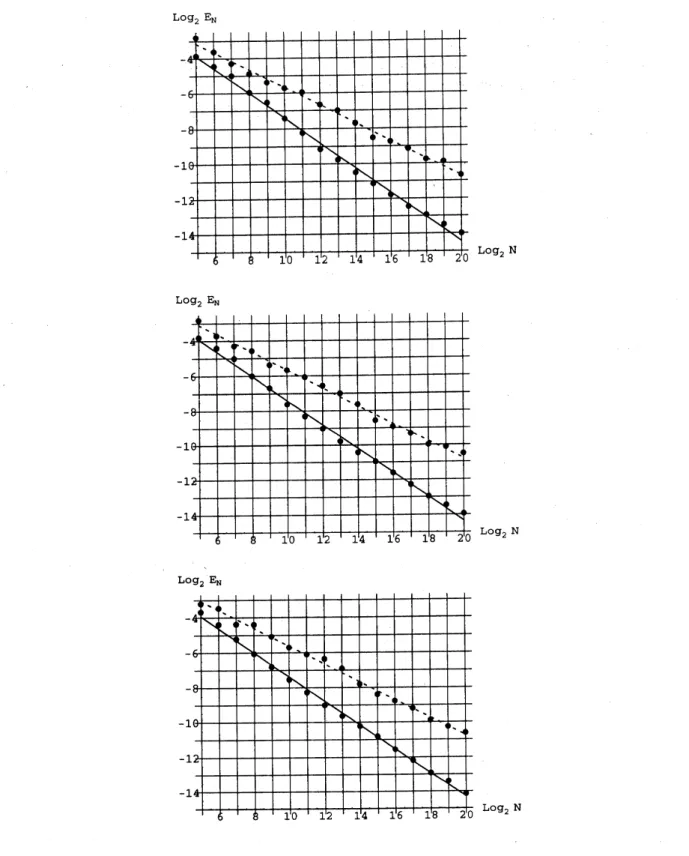
The QRW method is compared with the SRW method in Fig. 1. For all the calculations,

the number of simulated particles ranges from $N=32$ to $N=1,048,576$, with $N$ being

chosen as powers of two. In all cases, the averaged

error

is computed at each $N$, and a

line is fitted tothe log-log data to estimate the convergence rate. This

assumes

that

over

this range of $N$, the error may be modeled as $cN^{-d}$. One finds 1. For Euler’s method

$D_{N}( \mathrm{S}\mathrm{R}\mathrm{W})\approx\frac{0.64}{N^{0.50}}$, $D_{N}( \mathrm{Q}\mathrm{R}\mathrm{W})\approx\frac{0.77}{N^{0.70}}$. (29)

2. For Heun’s method

$D_{N}$(SRW) $\approx\frac{0.69}{N^{0.51}}$, _{$D_{N}$}(QRW) $\approx\frac{0.72}{N^{0.69}}$. .(30)

3. For Heun’s method with Strang splitting

$D_{N}( \mathrm{S}\mathrm{R}\mathrm{W})\approx\frac{0.70}{N^{0.51}}$, $D_{N}( \mathrm{Q}\mathrm{R}\mathrm{W})\approx\frac{0.72}{N^{0.69}}$. (31)

For each method, the quasi-random strategy produces sizable gains over pseud0-random

Monte Carlo. One easily sees the trend toward steady reduction oftlue error as

more

and

more

particles are used. Similar results have been observed for example in [4] for simple

diffusion problems.

3The

Burgers

equation

In this section we present aquasi-random _{walk method used} _to _{solve the} _quasilinear

diffusion equation

$\frac{\partial u}{\partial t}(x, t)+(u\frac{\partial u}{\partial x})(x, t)=\nu\frac{\partial^{2}u}{\partial x^{2}}(x, t)$, $x\in \mathrm{R}$, $t>0$, (32)

$u(x, 0)=u_{0}(x)$_, $x\in \mathrm{I}\mathrm{R}$,

(33)

with viscosity $\nu>0$_. The _equation _is _attributed _to _{Burgers aatd} _was _advanced _as _a

one

dimensional model for the Navier-Stokes equations. We

assume

that $u_{0}$ is constant

outside acompact set

$u_{0}(x)=\{$

$u_{-}$, if $x<-A$

$u_{+}$, if$x>A$. (34)

(7)

$\mathrm{L}\mathrm{o}g_{2}\mathrm{N}$

${\rm Log}_{2}\mathrm{N}$

Figure 1: Kolmogorov equation: Euler’s method (top), Heun’s method (middle) and

Heun’s method with Strang splitting (bottom): SRW (dotted line) $\mathrm{v}\mathrm{s}$

.

QRW (solid line)

averaged error

(8)

We follow [10] for the description of the random particle method for this equation. The

algorithm is based onaviscous splitting. We refer to [11] for information onthe numerical

solution ofconservation laws.

We choose integers $b\geq 2$, $m\geq 0$, we put $N:=b^{m}$ _and we _choose _aspatial

pa-rameter $h>0$. For the quasi-random walk, we need alow-discrepancy sequence $P=$

$\{\mathrm{p}_{0}, \mathrm{p}_{1}, \ldots\}\subset I^{2}$ satisfying (6) and (7). We suppose that the gradient

$u_{x}$ of the

s0-lution is approximated by acollection of weighted particles. The initial step function

approximation is given by

$u^{(0)}(x)=u_{-}+l \iota\sum_{0\leq j<N}\epsilon_{j}H(x-x_{j}^{(0)})$, (35)

where

$\epsilon_{j}=\pm 1$ and

$\sum_{0\leq j<N}\epsilon_{j}=\frac{u_{+}-u_{-}}{h}$. (36)

Here $x_{j}^{(0)}$ is the location and $h$ is the absolute strength ofthe

$j\mathrm{t}\mathrm{h}$particle.

Let $\triangle t$bethetime step andput

$t_{n}:=n\triangle t$, _{$u_{n}(x):=u(x, t_{n})$}. We denote thecomputed

solution after $n$ time steps as $u^{(n)}$,

$u^{(n)}(x)=u_{-}+l \iota\sum_{0\leq j<N}\epsilon_{j}H(x-x_{j}^{(n)})$. (37)

We assume that the particles have been labeled so that

$j<k\Rightarrow x_{j}^{(n)}\leq x_{k}^{(n)}$. and $\epsilon_{j}\geq\epsilon_{k}$. (38)

The approximate solution at time $t_{n+1}$ is obtained in two steps.

Step 1. Given particles at position $x_{j}^{(n)}$, $0\leq j<N$, we need to evolve the positions

in such away that the associated step function approximates _{the solution of the inviscid}

Burgers equation

$\frac{\partial u}{\partial t}(x, t)+(u\frac{\partial u}{\partial x}.)(x, t)=0$, $x\in \mathrm{R}$, _{$t>t_{n}$}, (39)

$u(x, t_{n})=u^{(n)}(x)$_, $x\in \mathrm{R}$. (40)

We solve the Riemann _{problems associated with each jump separately.} _Let

$[u^{(n)}]_{j}:=u^{(n)}(x_{j}^{(n)}+0)-u^{(n)}(x_{j}^{(n)}-0)$

be the strength of the jump at $x_{j}^{(n)}$.

$\bullet$ If $[u^{(n)}]j\leq 0$, then we have ashock and the speed of the

discontinuity is

$v_{j}^{(n)}:= \frac{1}{2}(u^{(n)}(x_{j}^{(n)}+0)+u^{(n)}(x_{j}^{(n)}-0))$ .

We define it as the velocity of the $j\mathrm{t}\mathrm{h}$ particle.

(9)

o If $[u^{(\mathrm{n})}]_{\ovalbox{\tt\small REJECT}}\ovalbox{\tt\small REJECT}>0$, then we have ararefaction wave. Assume that p A- q particles are

located at

\yen

$*7$

$x_{j}^{(n)}$ $=$ $x_{j+1}^{(n)}=\ldots=x_{j+p-1}^{(n)}$, with $\epsilon_{j}=\ldots=\epsilon j+p-1=+1$,

$x_{j}^{(n)}$ $=$ $x_{j+p}^{(n)}=\ldots=x_{j+p+q-1}^{(n)}$, with $\epsilon_{j+p}=\ldots=\epsilon j+\rho+_{l}‘-1=-1$.

We define the velocity of the $(j+k)\mathrm{t}\mathrm{h}$particle to be $v_{j+k}^{(n)}\cdot=\{$

$u^{(n)}(x_{j}^{(n)}-0)+(k. + \frac{1}{2})h$, if $0\leq k<p-q$ $u^{(n)}(x_{j}^{(n)}+0)$, if$p-q\leq k$. $<p+q$.

As time proceeds, the solutions start to interact: at this time we consider the

approxi-mating step function as new initial data. We set

$\delta t_{1}^{(n)}:=\min_{j,k}\{\frac{x_{k}^{(n)}-x_{j}^{(n)}}{v_{j}^{(n)}-v_{k}^{(n)}}$ : $x_{j}^{(n)}<x_{k}^{(n)}$ and $v_{j}^{(n)}>v_{k}^{(n)}\}$ ,

so that $t_{n}+\delta t_{1}^{(n)}$ is the first time ofintersectionof the trajectories ofat least two particles

that were at different positions at time $t_{n}$. For $t_{n}\leq t\leq t_{n}+\delta t_{1}^{(n)}$, the location ofthe

$j\mathrm{t}\mathrm{h}$

particle at time $t$ is

$x_{j}^{(n)}(t)=x_{j}^{(n)}+(t-t_{n})v_{j}^{(n)}$. (41)

If $\delta t_{1}^{(n)}\geq\triangle t$ we set

$x_{j}^{(n+1/2)}:=x_{j}^{(n)}(t_{n+1})$,

and we go to step 2, otherwise we replace $t_{n}$ by $t_{n}+\delta t_{1}^{(\tau\iota)}$ and we repeat step 1until we

reach $t_{n+1}$. Then

$u^{(n+1/2)}(x):=u_{-}+h \sum_{0\leq j<N}\epsilon_{j}H(x-x_{j}^{(n+1/2)})$.

Step 2. The next step involves solving the diffusion equation for $u_{x}$

$\frac{\partial u_{x}}{\partial t}(x, t)=\nu\frac{\partial^{2}u_{x}}{\partial x^{2}}(x, t)$ , $x\in \mathrm{R}$, $t>t_{n}$, (42)

$u_{x}(x, t_{n})=u_{x}^{(n+1/2)}(x)$, $x\in \mathrm{R}$

.

(43)

This is accomplished by adding aquasi-randomcomponent to the position of the particles.

We

assume

that the particles have been sorted in order of position:

$x_{0}^{(n+1/2)}\leq\ldots\leq x_{N-1}^{(n+1/2)}$. (44)

Then

$x_{\lfloor Np_{j,1}\rfloor}^{(n+1)}--x_{\lfloor Np_{j,1}\rfloor}^{(n+1/2)}+\sqrt{2\nu\triangle t}\Phi^{-1}(p_{j,2})$, $nN\leq j<(n+1)N$. (45)

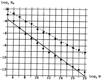
In order tocompare the performance of quasi-random walk (QRW) method described

above and standard random walk (SRW) employing pseud0-random numbers [10], both

(10)

${\rm Log}_{2}\mathrm{E}_{\mathrm{N}}$

Figure 2: Burgers equation: SRW (dotted line) $\mathrm{v}\mathrm{s}$. QRW (solid line) averaged

error

methods

are

used to solve amodel problem _{which has}

_an

_exact _{known solution. We}

_can

use the Cole-Hopftransformation to solve (32)-(33). If$u_{0}(x)=1-H(x)$,

we

obtain:

$u(x, t)=. \frac{\Phi((t-\tau)/\sqrt{2\nu t})\exp((t-2x)/4\nu)}{\Phi((t-x)/\sqrt{2\nu t})\exp((t-2x)/4\nu)+\Phi(x/\sqrt{2\nu t})}$

.

(46)

We choose $\nu=0.1$ and the solution is _computed _up _to _$T=1$ _{with atime} _step

$\triangle t=2^{-11}$. The QRW method utilizes _a _{$(0, 2)$}

-sequence of Faure in base 2. For all the

calculations, the number $N$ of particles ranges ffom _$N=32$ _to

$N=262,144$, with $N$

being chosen as _{powers of two. Figure 2shows alog-log} _plot _{of the} _averaged

_error

_(28).

The least-squares fit convergence rates

are

as follows:

$D_{N}( \mathrm{S}\mathrm{R}\mathrm{W})\approx\frac{1.31}{N^{0.54}}.$, $D_{N}( \mathrm{Q}\mathrm{R}\mathrm{W})\approx\frac{0.89}{N^{0.71}}$. (47)

We seethat the QRW method still clearly outperformsthe SRWmethod for thisexample,

although the problem being dealt with here is

more

complicated than simple diffusion

problem.

4Conclusion

In this paper we examine the use ofquasi-random _{sequences of}_{points in place} _of

pseud0-randompoints_{in random walk simulation of}_diffusion. _Two_problems _are _considered:

one-dimensional nonlinear reaction-diffusion equation and Burgers equation. The algorithm

has been tailored to fitin affactional step _{scheme. The results for the two}_problems_reveal

that quasi-Monte _{Carlo methods}

_can

_{be successfully} _applied _to _simple _{one-dimensional}

equations, producing

errors

which are _{smaller than standard random walk. Akey element}

in successfullyapplying the quasi-random sequencesis atechnique_{involving renumbering}

the particles after each time step

(11)

The algorithms arepresently suited for solving scalar, one-dimensionalequations. One

desirable extension would be to systems of equations such as the Hodgkin-Huxley

equa-tions. Afurther possible extension is to problems inmore than one space dimension, such

as the Navier-Stokes equations. On the theoretical side it will be especially interesting to

prove convergence of the schemes.

Acknowledgments

The author wishes to thank the organizer of the RIMS Symposium on Stochastic

Numer-$\mathrm{i}\mathrm{c}\mathrm{s}$, Professor Ogawa S. for inviting him to speak.

Further he gratefully acknowledges the Centre Grenobloisde Calcul Vectoriel du

Com-missariat \‘a l’Energie Atomique for allowing him to use its computer facilities.

References

[1] A.J. Chorin, Numericalmethods

_for

use in combustionmodeling, Computing Methods

in Applied Sciences and Engineering (R. Glowinski and J.L. Lions, eds.), North

Holland, Amsterdam, 1980, pP. 229-236.

[2] H. Faure, Discr\’epance de suites associ\’ees \‘a un syst\‘eme de num\’eration (en dimension

s), Acta Arith. 41 (1982), 337-351.

[3] A.F. Ghoniem and F.S. Sherman,

Grid-free

simulation

of diffusion

using random

walk methods, J. Comput. Phys. 61 (1985), 1-37.

[4] C. Lecot and F. El Khettabi, Quasi-Monte Carlo simulation

_of

diffusion, J.

Com-plexity 15 (1999), 342-359.

[5] C. Lecot and A. Koudiraty,

_Grid-free

simulation

_of

convection-diffusion, Monte

Carlo and Quasi-Monte Carlo Methods 1998 (H. Niederreiter and J. Spanier, eds.),

Springer, Berlin, 2000, pP. 311-325.

[6] H. Niederreiter, Random Number Generation and Quasi-Monte Carlo Methods,

SIAM, Philadelphia, 1992.

[7] H. Niederreiter and J. Spanier $(\mathrm{e}\mathrm{d}\mathrm{s}.)\grave,$ Monte Carlo and Quasi-Monte Carlo Methods

1998, Springer, Berlin, 2000.

[8] S. Ogawa, On a robustness

_of

the random particle method, Monte Carlo Methods

Appl. 2(1996), 175-189.

[9] E.G. Puckett, Convergence

_of

a random particle method to solutions

of

the

Kol-mogorov equation $u_{t}=\nu u_{xx}+u(1-u)$, Math. Comput. 52 (1989) 615-645.

[10] S. Roberts, Convergence

_of

a random walk method

_for

the Burgers equation, Math.

Comput. 52 (1989), 647-673.

[11] J.W. Thomas, Numerical Partial

_Differential

Equations, Conservation Laws and

El-liptic Equations, Springer, New York, 1999