A NUMERICAL APPROACH TO THE DISCRETE MORSE SEMIFLOW HIDETOSHI
YOSHIUCHI1
(吉内栄利) SEIROOMATA2
(小俣正朗)$0$
.
AbstractIn thispaper, we treat a numericalanalysis of discrete Morse semiflows for energy minimizing harmonic mapping. Discrete Morse semiflows were introduced by Rektorys and Kikuchi for
ap-proximating solution of heat equations associated to variational problems. Inspired by Kikuchi’s
results, several authors use this method for constructing weak solutions of parabolic equations.
We apply this flow to the numerical analysis and develop energy minimizing algorithmfor solving
approximate heat equation.
1. Introduction
In this paper, a numerical analysis of discrete Morse semiflows for harmonic mapping from $\mathrm{B}^{3}$
to $S^{2}$ isstudied. Thisis considered to be the approximationof the heat flow of thefollowingelliptic
problem: Minimize the functional;
$\mathcal{I}(u)=\int_{\mathrm{B}^{3}}|\nabla u|^{2}dx$, $u|_{\partial \mathrm{B}^{3}}=\varphi$ in $H_{\varphi}^{1}(\mathrm{B}^{3};s^{2})$
.
Some authors have studied this problem from a numerical point of view. (See [A1] for example.)
Here, we present an new algorithm which use the discrete Morse semiflow for solving heat
equation. For this purpose, we introduced thefollowing time-semidiscretized functional;
$J_{m}^{h}(u)= \int_{\mathrm{B}^{3}}\frac{|u-u_{m-1}|^{2}}{h}dc^{n}+\mathcal{I}(u)$, $(m=1,2, \cdots)$
.
(1.1)The$\mathrm{p}_{\mathrm{I}\mathrm{O}\mathrm{C}}\mathrm{e}\mathrm{d}\mathrm{u}\mathrm{r}\mathrm{e}$ of determining sequence is asthe folowing: Let $u_{0}$ be a given initialdata satisfying
$u_{\mathrm{O}}\in \mathcal{K}$, and $\mathcal{I}(u_{\mathrm{O}})<\infty$,
where $\mathcal{K}$ is an admissible function space of the original functional$\mathcal{I}$(In this case $\mathcal{K}=H_{\varphi}^{1}(\mathrm{B}3;^{s^{2}})$). Taking $u_{0}$ as $u_{m-1}$ ($m=1$ is assumed) in $\mathcal{K}$, we define a minimizer
$u_{1}$ of$J_{1}$
.
Inductively wedefine$u_{m}$ by the minimizer of $J_{m}$ in $\mathcal{K}$
.
We will call $\{u_{m}\}$ the discrete Morse semiflow.Since the minimizers $\{u_{m}\}$ depend on the positive constant $h$, we should write $\{u_{m}^{h}\}$
.
But sometimes we use the notation $\{u_{m}\}$ when no confusions may occur.(1) ULVAC corporation: Hagisono 2500, Chigasaki, 253 Japan.
(2) Department of Mathematics, Faculty of Science, Kanazawa University: Kakuma-machi,
Kanaz$\mathrm{a}\mathrm{w}\mathrm{a}$, 920-11 Japan.
Partly supported by the $\mathrm{G}\mathrm{r}\mathrm{a}\mathrm{n}\mathrm{t}_{\mathrm{S}}-\mathrm{i}\mathrm{n}$-Aid for Encouragement of Young Scientist, The Ministry of
Using this approach, Kikuchi constructed solutions ofparabolicequations associated to a
varia-tional functionalofharmonic map type in [K]. Nagasawa and Omata havestudied the asymptotic
behavior of this flow on somefree boundary problems. (See [NO1] and $[\mathrm{N}\mathrm{O}2].$) On theother hand,
Bethuel, Coron, Ghidaglia and Soyeur ([BCGS]) also showed the existence of the Morse semiflow
associated to relaxedenergies for harmonic mapping by this $\mathrm{p}\mathrm{r}\mathrm{o}\mathrm{c}\mathrm{e}\mathrm{d}\mathrm{u}\mathrm{I}\mathrm{e}$
.
2. Main property of the discrete Morse semiflow
Apart fiom the harmonic mapping, we here mention the basic property of the discrete Morse
semiflow. Among almost all quadratic functional$\mathcal{F}(u)$, we can determine the discrete Morse
semi-flow is the same way as in section 1 and they have the folowing property:
$J_{m}^{h}(u_{m}^{h}) \equiv\int_{\Omega}\frac{|u_{m}^{h}-u_{m-1}h|^{2}}{h}dx+\mathcal{F}(u_{m})h\leq J_{m}^{h}(u_{m}^{h}-1)\equiv \mathcal{F}(u^{h})m-1$
’
therefoIe
$\int_{\Omega}\frac{|u_{m}^{h}-u^{h}m-1|^{2}}{h}\leq \mathcal{F}(u_{m-1})h-\mathcal{F}(u_{m}h)$
.
(2.1)Summing upfrom $m=1$ to $N$, the following estimate holds:
$F(u_{N}^{h})+ \sum_{m=1}^{N}\int_{\Omega}\frac{|u_{m}^{h}-u_{m-1}^{h}|^{2}}{h}d_{X}\leq \mathcal{F}(u_{0})$
.
(2.2)This is a basic and important estimate of this flow. Many $\mathrm{p}_{\mathrm{I}\mathrm{O}}\mathrm{p}\mathrm{e}\mathrm{I}\mathrm{t}\mathrm{i}\mathrm{e}\mathrm{s}$ is to be obtained from (2.2).
Wecan Iegard suchsequences ofminimizers as $\mathrm{a}\mathrm{p}\mathrm{p}_{\mathrm{I}\mathrm{O}}\mathrm{x}\mathrm{i}\mathrm{m}\mathrm{a}\mathrm{c}\mathrm{e}$solutions of the heat equation. For
this, we will introduce following two functions.
DEFINITION 2.1. We deRn$e$functions $\overline{u}^{h}$ and $u^{h}$ on
$\Omega \mathrm{x}(0, \infty)$ by $\overline{u}^{h}(X, t)=u^{h}m(x)$
$u^{h}(X, t)= \frac{t-(m-1)h}{h}u_{m}^{hh}(x)+\frac{mh-t}{h}um-1(x)$
for$(x, t)\in\Omega \mathrm{x}((m-1)h, mh]$
.
It is easy to see that the functions above satisfy the folowing relations:
$\frac{\partial u^{h}(x,t)}{\partial t}=\delta F\overline{u}^{h}(X, t)$ in some
weak sensein $\Omega \mathrm{x}\bigcup_{m=2}((m-1)\infty h, mh)$
$\overline{u}^{h}(x, t)=u^{h}(x, t)=u_{0}(X)$ on $\partial\Omega$
$u^{h}(x, 0)=u_{0}(X)$ in $\Omega$
.
Here, we investigate the convergence theory when $h$ tends to zero. We can easily obtain the
THBOREM 2.3. If$F$ is corecive, then the following norms are uniformly bounded with
respect to $h$
.
$|| \frac{\partial u^{h}}{\partial t}||_{L^{2}(}(0,\infty)\mathrm{X}\Omega)$
’ $||\nabla\overline{u}^{h}||L\infty((0,\infty);L2(\Omega))$’ $||\nabla u^{h}||L\infty((0,\infty);L2(\Omega))$’
$||u^{h}||_{L}\infty((0,\infty);L^{2}(\Omega))$
’ $||\overline{u}^{h}||_{L}\infty((0,\infty);L2(\Omega))$’ $||u^{h}||W1,2((0,T)\mathrm{X}\Omega)$ (for
au
$T>0$). THEOREM 2.4. Thereexists a $s\mathrm{u}$bsequence, such that$\overline{u}^{h}arrow u$ weakIy starin $L^{\infty}((0, \infty);L^{2}(\Omega))$ (2.3) $u^{h}arrow u$ weaklyin $W^{1,2}((0,T)\mathrm{x}\Omega)$ (2.4) $u^{h}arrow u$ strongly in $L^{2}((0,T)\mathrm{X}\Omega)$ (2.5)
$\overline{u}^{h}arrow u$ stronglyin $L^{2}((0,T)\mathrm{X}\Omega)$
.
(2.6)These propertiesfollow from the basic estimate (2.2) and the following theorem.
THEOREM 2.5. Thefunction $\overline{u}^{h}$
and$u^{h}$ converge to thesame function $u$in thefollowing sense for any$T$:
$\overline{u}^{h}arrow u$ weaklyin $L^{2}(\Omega \mathrm{x}(0,T))$ $u^{h}arrow u$ weaklyin $H^{1}(\Omega \mathrm{x}(0,T))$
and$s$tron$gl\mathrm{y}$in $L^{2}(\Omega \mathrm{x}(0,T))$
.
Proof. FIom (2.2), we have
$\int_{\Omega}|\nabla\overline{u}^{h}(X, Nh)|2dx+\int_{0}^{Nh}\int_{\Omega}|\frac{\partial u^{h}}{\partial t}(x,t)|2dx$
$\leq \mathcal{F}(u_{0})$
.
It implies that $\{\overline{u}^{h}\}_{h>}0$ and $\{u^{h}\}_{h>}0$ are bounded sets in $L^{2}(\Omega \mathrm{x}(0,T))$ and $H^{1}(\Omega\cross(0,T))$
respectively for any $T>0$
.
Therefore we can extract a subsequence $\{h_{j}\}$ such that $h_{j}\downarrow \mathrm{O}$ and$\overline{u}^{h_{j}}arrow u$ weakly in $L^{2}(\Omega \mathrm{x}(0,T))$
$u^{h_{j}}arrow v$ weakly in $H^{1}(\Omega \mathrm{x}(0, T))$
andstrongly in $L^{2}(\Omega \mathrm{x}(0,T))$
as $jarrow\infty$
.
It folows from $|u^{h}- \overline{u}^{h}|\leq|\frac{\partial u^{\mathrm{h}}}{\partial t}|$that
$\int_{0}^{T}\int_{\Omega}|u^{h}-\overline{u}^{h}|^{2}d_{Xdt}\leq h^{2}\int_{0}^{\infty}\int_{\Omega}|\frac{\partial u^{h}}{\partial t}|^{2}dxdt$
$\leq h^{2}\mathcal{F}(u_{0})arrow 0$ as $h\downarrow 0$, which shows $u=v$
.
I
3. Recent results on the Harmonic Mapping into Sphere
Bethuel, Coron, Ghidaglia and Soyeur constIucted weak heat flows related to the Harmonic
THEOREM 3.1. Let $u_{0}$ and $\gamma$ belong to $H^{1}(\mathrm{B}^{3};s^{2})$ lrith $u_{0}=\gamma$ on
$\partial \mathrm{B}^{3}$
.
There exists a
weaksolution to
$\frac{\partial u}{\partial t}-\triangle u=u|\nabla u|^{2}$ (3.1)
$u(x, t)=\gamma(x)$, $t>0$, $x\in\partial \mathrm{B}^{3}$ (3.2)
$u(x, 0)=u_{0}(x)$, $x\in \mathrm{B}^{3}$
.
(3.3)4. Numerical analysis
We mention here a minimizing algorithm $\check{\mathrm{u}}$
sed in this paper. The minimizing algorithm means
some procedure that determine sequence ofcomparison function which will converge to the
min-imizer. Our method is $\mathrm{b}\mathrm{a}s$ed on the simplex search method which is one of the
finite element
method. Thescheme of the simplex searchmethod is as folows: (1) Discretizethe domain intothe
suitable elements which is calledfinite element. (We willassume that the domainis divided into$M$
elements with $N$ nodes.) (2) Approximate the comparison function by using the piecewise linear
function which is coincide with original compaIison function on nodal points. By this
approxima-tion, we can Iegard the elements of $R^{N}$ as the approximate comparison function. (3) Generate a
simplex in $R^{N}$
.
The simplex consist of$N+1\mathrm{v}\mathrm{e}\mathrm{I}\mathrm{t}\mathrm{i}_{\mathrm{C}}\mathrm{e}\mathrm{S}$.
(4) Calculatethe value of the functional ateach vertex of the simplex, and find the maximizer($\mathrm{t}\mathrm{h}\mathrm{e}$vertex
where the value of the functionalis
the largest). Then, movethemaximizingpoint to the oppositeside of$\mathrm{h}\mathrm{y}\mathrm{P}^{\mathrm{e}\mathrm{I}}\mathrm{P}\mathrm{l}\mathrm{a}\mathrm{n}\mathrm{e}$ which isspanned
by another vertices. By this procedure, we can make a new simplex. (5) Repeat this step up to
satisfy the given terminate conditions.
Throughout these procedures, we expect to find an approximate minimizer.
We $\mathrm{p}_{\mathrm{I}}\mathrm{o}\mathrm{c}\mathrm{e}\mathrm{e}\mathrm{d}$ discretization along to this algorithm using finite elements. Firstly, split $\mathrm{B}^{3}$ into
$M$ small finite elements(tetrahedron) with $N$ nodes. In order to use the simplex search method, we choose values of all nodal points. Secondly, approximate a comparison function $u$ by thelinear
function,
$\overline{u}=\{\tilde{u}_{1},\tilde{u}_{2},\tilde{u}_{3}\}$
$\tilde{u}_{1}=A_{1}x_{1}+B_{:}x_{2}+C_{i^{X_{3}}}+D_{*}$,
in anfinite element, which coincidewith the givendata on the nodal point. ($A_{\dot{*}},$$B_{i},$ $c_{:}$, and $D_{i}$ are
uniquely determined by the value at each nodal point.)
Thirdly, calculate the value of the functional for the approximate function. For calculation, we
introduce the folowingpenalized variational problem: Minimize
$\tilde{J}_{m}^{h}(u)=\int_{\mathrm{B}^{3}}(\frac{|u-u_{m-1}|^{2}}{h}+|\nabla u|2+\frac{1}{\epsilon}(|u|^{2}-1)2)dx$ , (4.1)
We use the folowing discretization for $\tilde{J}_{m}^{h}(u)$:
$\int_{\mathrm{B}^{3}}\frac{|u-u_{m-1}|^{2}}{h}dx=\frac{1}{h}\sum k=1M(.\sum_{1=1}^{3}(=\sum_{l1}^{16}(u_{1}s.,uk,lb)2\mathrm{x}(vol_{k/16)}\mathrm{I})$ (4.2)
$\int_{\mathrm{B}^{3}}|\nabla u|^{2}dX=\sum^{M}k=1(_{1j}.,\sum_{=1}^{3}(\frac{\partial\tilde{u}_{1}}{\partial x_{\mathrm{j}}}.)^{2}\cross vol_{k})$
$= \sum_{k=1}^{M}(.\sum_{1=1}^{3}(A2.,B.2,+|k+|kc^{2}.k)*,\mathrm{x}vol_{k)}$ (4.3)
$\int_{\mathrm{B}^{3}}\frac{1}{\epsilon}(|u|^{2}-1)2dX=\sum_{=j1}^{N}.\sum_{1=1}\frac{1}{\epsilon}((u:,j)^{2}-1)^{2}3$ (4.4)
where $u:,j$ and $u:,j,m-1$ denote the value of the function $u_{1}.(x)$ and $u:,m-1(X)$ at the jth node
respectively, $vol_{k}$ denotes the volume of the $k\mathrm{t}\mathrm{h}$ element and $A_{:,k},$$B:,,$${}_{k}C:,k$ denote the coefficients
of the approximated function $\tilde{u}:(x)$on $k\mathrm{t}\mathrm{h}$ element. For the term (4.2), we divide an element into
16 subelements and
assume
that the function $|u-u_{m-1}|2$ is linear on the each subelement. $u_{1}^{su_{k}b}.,,\iota$denotes the the value of the approximated $|ui-ui,m-1|^{2}(i=1,2,3)$ on the $l\mathrm{t}\mathrm{h}$ subelement in the
$k\mathrm{t}\mathrm{h}$ element.
5. Result
We calculat$e,$ $\mathrm{h}\mathrm{e}\iota \mathrm{e}$, both linear(without term 4.4) and nonlinear cases. In the linear case, we
adopt the folowing conditions.
(1) Initial data:
$u_{0}(x)=f^{-}z1(x)$ where $f_{z}(x)=(1-|x|)z+x$, $\exists z\in \mathrm{B}^{3}$
.
(2) Boundary condition:
$u_{m}(x)|_{\partial \mathrm{B}}s=i.d$
.
$(m=1,2, \cdots)$ (3) Parameters:$(\epsilon=+\infty)$, $h=0.1$ $z=(0,0,0.9)$
.
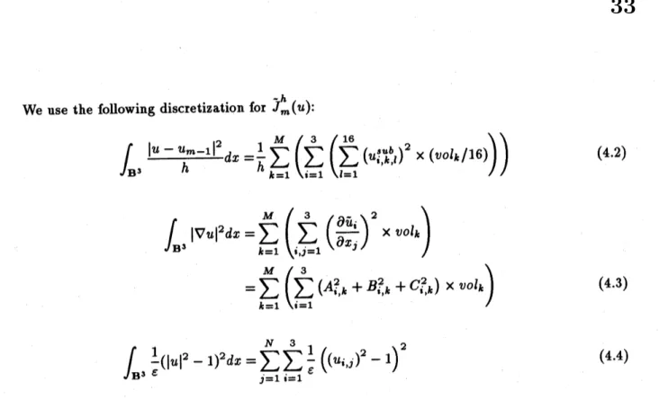
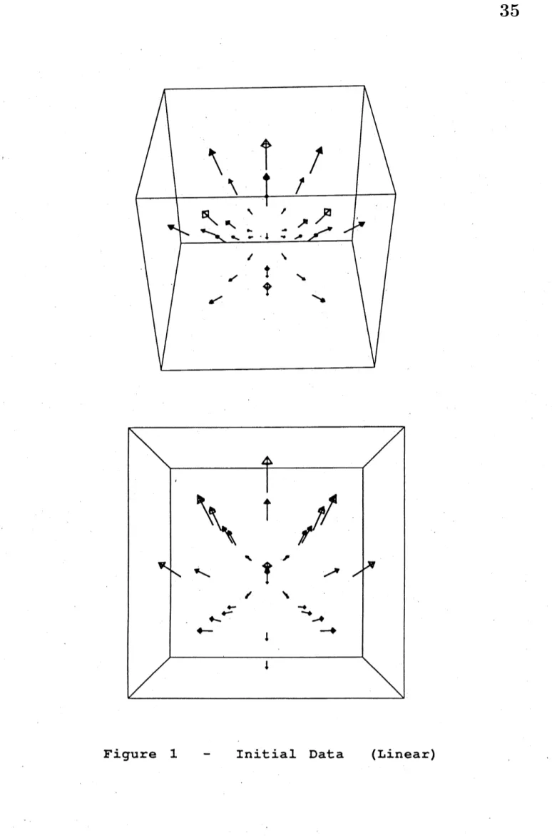
Figure 1 and 2 denotes $u_{0}$ and $u_{1}$ respectively in the linear case. In figures, arrows denotes
vector field inside of$\mathrm{B}^{3}$
.
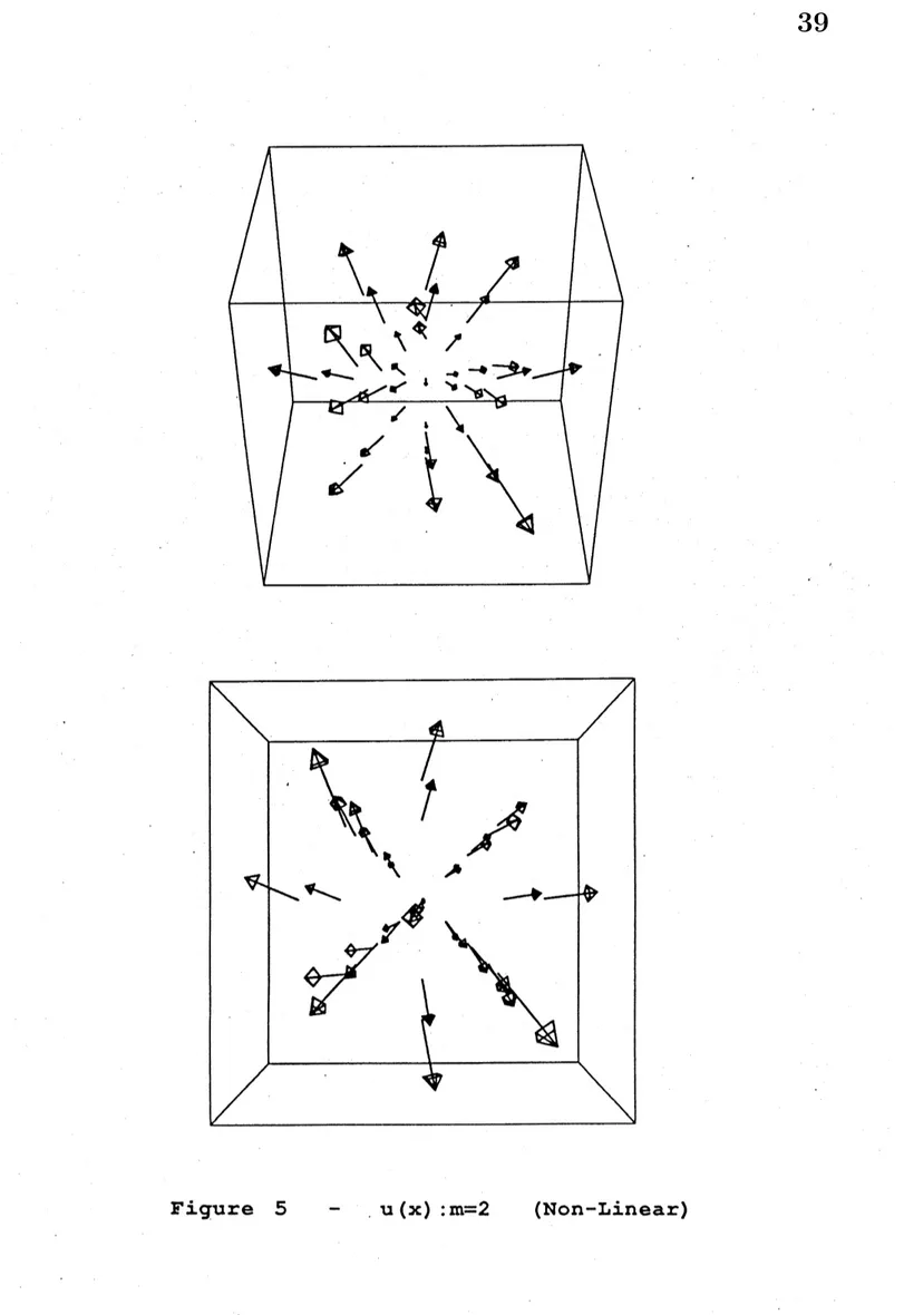
(Boundary data are omitted.)In the nonlinear case, we calculate this under the folowing conditions.
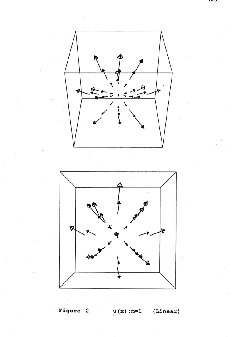
(1) Initial data:
$u_{\mathrm{O}}(_{X})=p(f_{z}^{-1}(x))$ where $f_{z}(_{X})=(1-|x|)Z+x$,
$\exists z\in \mathrm{B}^{3}$
(2) Boundary condition:
$u_{m}(x)|_{\partial}\mathrm{B}3=i.d$
.
$(m=1,2, \cdots)$ (3) Parameters:$\epsilon=0.01$, $h=0.1$ $z=(0,0,0.9)$
.
Figure 3, 4 and 5 denotes $u_{0},$ $u_{1}$ and $u_{2}$ respectively. Also, arrows denotes vector field. Because $h$ relatively is large, the singular points moves
very fast in the first time step. It is
verynatuIal toconsider that the motion of thesingular points depends on the parameter $h$ and $\epsilon$
.
Thus, we should calculate carefuly changing theseparameters. But unfortunately, we do not have
enough computer poweI. Up to now, we only calculate the case when $h=0.1$ and $\epsilon=0.01$
.
WeFigure
2
–$\mathrm{u}\backslash (\mathrm{x})$
:
$\mathrm{m}=1$
Acknowledgement
We greatly thank Prof. N.Kikuchi at Keio University for introducing us to this approach.
References
[A1] F.Alouges, “An energy-decreasing algorithm
for
harmonic map”,in “Nematics–Mathematical and PhysicalAspects”, ed.: J.-M.Coron, J.-M.Ghidaglia, F.H\’elein, NATO Adv. Sci. Inst. Ser. C: Math. Phys. Sci. 332, Kluwer Acad. Publ., Dordrecht- Boston- London, 1991, 195-198. [BCGS] F.Bethuel- $\mathrm{J}.- \mathrm{M}.\mathrm{c}_{\mathrm{o}\mathrm{I}\mathrm{o}\mathrm{n}}- \mathrm{J}.- \mathrm{M}.\mathrm{G}\mathrm{h}\mathrm{i}\mathrm{d}\mathrm{a}\mathrm{g}\mathrm{l}\mathrm{i}\mathrm{a}- \mathrm{A}.\mathrm{S}_{0}\mathrm{y}\mathrm{e}\mathrm{u}\mathrm{I}$ , “Heatflows
and relaxed energiesfor
har-monic maps, Nonlinear diffusionequations and their equihbrium states, 3. (Progressin
nonlin-ear differential equations and their applications, 7.) Birkh\"auser, Boston, Basel, Berlin(1992),
99-109.
[K] N.Kikuchi, “An approach to the construction
of
Morseflows for
variational functionals”, in“Nematics–Mathematical and Physical Aspects”, ed.: J.-M.Coron, J.-M.Ghidaglia, F.H\’elein, NATO Adv. Sci. Inst. Ser. C: Math. Phys. Sci. 332, Kluwer Acad. Publ., Dordrecht
-Boston- London, 1991, 195-198.
[NO1] T.Nagasawa- S.Omata, “Discrete Morse
semiflows of
afunctional
withfree
boundary”, Adv.Math. Sci. Appl. 2 (1993), 147-187.
[NO2] T.Nagasawa-S.Omata, “Discrete Morse
semifiows
and their convergenceof
afunctional
withfree
boundary”, in Nonlinear PaItial Differential Equations- PIoceedings of the InternationalConference Zhejiang University, June 1992, Ed. Dong Guangchang and Lin Fanghua,
Interna-tional Academic Publishers, Beijing 205-213 (1993).
[Re] K.Rektorys, “On application
of
direct variational methds to the solutionof
parabolic boundaryvalue problems