SHORT GEODESICS AND END INVARIANTS (Comprehensive Research on Complex Dynamical Systems and Related Fields)

SHORT GEODESICS AND END INVARIANTS

YAIR N. MINSKY

Even topologically simple hyperbolic 3-manifolds can have very intricate geometry. Consider in particular a closed surface $S$ ofgenus 2

or

more, and

the product $N=S\cross \mathrm{R}$. This 3-manifold admits

a

large family of complete,

infinite-volume hyperbolic metrics, corresponding to faithfulrepresentations

$\rho:\pi_{1}(S)arrow \mathrm{P}\mathrm{S}\mathrm{L}_{2}(\mathrm{C})$ with discrete image.

The geometries of $N$ are very different from the product structure that

its topology would suggest. Typically, $N$ contains a complicated pattern

of “thin” and $\zeta$

‘thick” parts. The thin parts are collar neighborhoods of very short geodesics, typically infinitelymany. Each one, called

a

$‘(\mathrm{M}\mathrm{a}\mathrm{r}\mathrm{g}\mathrm{u}\mathrm{l}\mathrm{i}\mathrm{s}$

tube”, has a well-understoodshape, but the wayin whichthese

are

arranged

in $N$, and in particular the identities of the short geodesics as elements of

the fundamental group, are still something of a mystery.

This issue _{is closely related to the basic classification conjecture} associ-ated with these manifolds, Thurston’s $‘(\mathrm{e}\mathrm{n}\mathrm{d}\mathrm{i}\mathrm{n}\mathrm{g}$ lamination conjecture”. This

conjecture states that certain asymptotic invariants of the geometry of $N$,

called ending invariants, in fact determine $N$ completely. (Actually the

classification of hyperbolic structures for any manifold with incompressible

boundary reduces to this case, by restriction to boundary subgroups.)

In this expository paper we will focus on the following question: What

information do the ending invariants give about the presence of very short geodesics in the manifold? We will summarize and discuss the theorem below, part of whose proofappears in [40] and part of which will be in [33],

as

well

as

a few conjectures.

Bounded Geometry Theorem. Let $S$ be a closed surface, and consider a Kleinian

_surface

group $\rho$ : $\pi_{\dot{1}}(S)arrow PSL_{2}(\mathrm{C})$ with no externally short

curves, and ending invariants $\iota/+andu_{-}$. Then

$\inf_{\gamma\in\pi_{1(S)}}\ell_{\rho}(\gamma)>0\Leftrightarrow\sup_{Y\subset S}d_{Y}(\nu_{+}, \nu_{-})<\infty$.

Here the supremum is over proper essential isotopy classes of subsurfaces in $S$, and the quantities $d_{Y}$$(\nu_{+}, \nu-)$, called “projection coefficients”, are defined in Section 1.4. The quantity $\ell_{\rho}(\gamma)$ is the translation distance of$\rho(\gamma)$

in $\mathrm{H}^{3}$

, or the length of the closed geodesic associated to $\gamma$ in the 3-manifold.

(The conditionon externally short

curves

is not really necessary-it is added to simplify the other definitions and discussions–see

_{\S 1.1}

below).

Part ofour goal is to advertise a combinatorial object known as the com-plex

_of

curves on a surface, as a tool for studying the geometry of hyperbolic 3-manifolds. This object is used for definining the coefficients $d_{Y}$, and in

general it encodes something about the structure of the set of simple loops

on

a surface. In particular, face transitions between simplices in this complex correspond to elementary moves on pants decompositions of $S$, and these

in turn correspond to homotopies between elementary pleated surfaces in a hyperbolic 3-manifold. The interaction between the combinatorial and geo-metric aspects of these

moves

is our main object of study, and

seems

to be worthy of further consideration.

1. DEFINITIONS

1.1. Surface

groups

and ending laminations. Let $S$ be a closed surface ofgenus$g\geq 2$. A Kleinian

surface

group willbe arepresentation$\rho$ : $\pi_{1}(S)arrow$ $\mathrm{P}\mathrm{S}\mathrm{L}_{2}(\mathrm{C})$, discrete and faithful. The quotient $\mathrm{H}^{3}/\rho(\pi_{1}(S))$ is denoted $N_{\rho}$,

and

comes

equipped with a homotopy class of homotopy equivalences $Sarrow$

$N_{\rho}$, determined by $\rho$. In fact $N_{\rho}$ is homeomorphic to $S\cross \mathrm{R}$, by Thurston’s

theory of tame ends [45] and Bonahon’s Tameness theorem [7].

We can associate to $\rho$ two ending invariants $\nu$-and $u_{+}$, which we will

describe in the specialcase that$\rho$ has noparabolics (see also [36] andOhshika

[42]$)$.

Let $C(N_{\rho})$ be the convex core of $N_{\rho}$, the smallest

convex

submanifold

whose inclusion is a homotopy equivalence. Fixing an orientation on $S$ and

$N_{\rho}$, there is anorientation-preserving homeomorphism of$N_{\rho}$ to $S\cross \mathrm{R}$taking

$C(N_{\rho})$ onto exactly one of $S\cross \mathrm{R},$ $S\cross[0, \infty),$ $S\cross(-\infty, 1]$

or

$S\cross[0,1]$.

The end of $N$ defined by neighborhoods $S\cross(a, \infty)$ is called $e_{+}$, and

the one defined by $S\cross(-\infty, a)$ is called $e_{-}$. If an $\mathrm{e}\mathrm{n}\mathrm{d}$)

$\mathrm{s}$ neighborhoods all

meet the convex hull it is called geometrically infinite, and otherwise it is geometrically

_finite.

Suppose$e_{+}$ is geometrically finite. Then the component

$\partial_{+}(C(N_{\rho}))$ corresponding to $S\cross\{1\}$ is a

convex

surface, and its exterior

$S\cross(1, \infty)$ develops out to a

$\zeta$

‘conformal structure at infinity” on $S$, which we call $\nu_{+}$. (This surface is obtained from the action of $\rho(\pi_{1}(S)$ on the

Riemann sphere). We define $\nu_{-}$ in the same way when $e_{-}$ is geometrically

finite.

Thurston pointed out that boundary $\partial_{+}(C(N_{\rho}))$ is itself a hyperbolic surface; let us call its structure $\nu_{+}’$. A theorem of Sullivan (proofin

Epstein-Marden [15]$)$ states that $\nu_{+}’$ and $\nu_{+}$ differ by a uniformly bilipschitz

distor-tion.

To describe the invariant ofa geometrically infinite end

we

need to briefly recall the notion of a geodesic lamination. Fixing a hyperbolic metric on $S$, a geodesic lamination is a closed subset of $S$ foliated by geodesics. Let

$\mathcal{G}\mathcal{L}(S)$ denote the set of all of these. A measured lamination is a geodesic

lamination equipped with a Borel

measure on

transverse arcs, invariant un-der transverse isotopy. The space $\mathcal{M}\mathcal{L}(S)$ of measured laminations admits

the supporting geodesic laminations, this is related to but not quite the same as the topology of Hausdorff

convergence.

However the difference will not be important to us here. Simple closed geodesics with positive weights

are

dense in $\mathcal{M}\mathcal{L}(S)$, and

we

will consider geodesic laminations obtained

as

supports of limits in $\mathcal{M}\mathcal{L}(S)$ of sequences of simple closed

curves.

Finally

we remark that the choice of metric on $S$ is irrelevant,

as

any other choice yields naturally isomorphic spaces of laminations. For

more

details on this topic see Bonahon $[5, 6]$, Canary-Epstein-Green [13]

$)$ or Casson-Bleiler [14].

If $e_{+}$ is geometrically infinite then the

convex

hull contains an infinite

sequence of closed geodesics $\gamma_{n}$, all homotopic to simple closed loops on $S$,

and eventually contained in $S\cross(a, \infty)$ for any $a$. This is a theorem of

Bonahon, and Thurston (previously) showed that for such

a

sequence the

curves

on $S$must convergein the

sense

of the previous paragraph to aunique

geodesic laminationon $S$. We callthis lamination

$\nu_{+}$, the ending lamination

of $e_{+}$. The corresponding discussion for $e_{L}$ gives $\nu_{-}$.

Finally let us define thetechnicalsimplifyingcondition in the statement of the Bounded Geometry Theorem. Call a

curve

$\gamma$ in $S$ externally short, with

respect to

a

representation $\rho$, if it is either parabolic

or

has length less than

$\epsilon_{1}$ with respect to the structures $\iota/$-and

$\nu_{+}$ (if these

are

not laminations),

where $\epsilon_{1}$ is some fixed constant small enough that there exist hyperbolic

structures on $S$ with no curves of length less than

$\epsilon_{1}$. Note in particular

that if $\rho$ has two degenerate ends then it automatically has

no

externally

short

curves.

1.2. Pleated surfaces. Apleated

_surface

isamap $f$

:

$Sarrow N$together with ahyperbolicmetricon $S$, written$\sigma_{f}$ and called the inducedmetric, anda $\sigma_{f^{-}}$

geodesic lamination $\lambda$ on $S$, called the pleating locus,

so

that the following

holds: $f$ is length-preserving

on

paths, maps leaves of$\lambda$ to geodesics, and is

totally geodesic onthe complement of$\lambda$. These

were

introducedbyThurston

[45], and

we

will

see some

explicit examples in

_{\S 4.1.}

It is a consequence of the work of Thurston and Bonahon that a geo-metrically infinite end of a surface group $\rho$ admits pleated surfaces in the

homotopy class of $\rho$ contained in any neighborhood of the end. The

pleat-ing loci of these surfaces must converge to the ending lamination, and their hyperbolic structures

converge

to this lamination in Thurston’s compactifi-cation of the Teichm\"uller space.

1.3. Complexes of

arcs

and

curves:

Let $Z$ be

a

compact finite genus surface, possibly with boundary. If $Z$ is not

an

annulus, define _{$A_{0}(Z)$} to be the set of essential homotopy classes of simple closed

curves or

properly embedded

arcs

in $Z$. Here “homotopy class” means free homotopy for closed curves, and homotopy rel $\partial Z$ forarcs. “Essential” means the homotopy class

does not contain the constant map

or

a map into the boundary. If $Z$ is an

annulus, we make the same definition except that homotopy for arcs is rel

We can extend $A_{0}$ to

a

simplicial complex $A(Z)$ by letting a $k$-simplex be

any $(k+1)$-tuple $[v_{0}, \ldots, v_{k}]$ with $v_{i}\in A_{0}(Z)$ distinct and having pairwise

disjoint representatives.

Let $A_{i}(Z)$ denote the $i$-skeleton of $A(Z)$, and let $C(Z)$ denote the

sub-complex spanned by vertices corresponding to simple closed

curves.

This is the “complex of

curves

of $Z$”.

Ifwe put a path metric

on

$A(Z)$ making every simplex regular Euclidean

of sidelength 1, then it is clearly quasi-isometric to its 1-skeleton. It is also quasi-isometric to $C(S)$ except inafew simple

cases

when $C(S)$ has no edges.

When $\partial Z=\emptyset$, of

course

$A=C$.

It is anice exercise to compute $A(Z)$ exactly for $Z$ a one-holed torus, and

we

leave this to the reader. The

answer

is closely related to the Farey graph in the plane–see [37].

Fix our closed surface $S$ and let $\mathcal{G}\mathcal{L}(S)$ denote the set of geodesic

lamina-tions on $S$ (note that _{$A_{0}(S)=C_{0}(S)$} can identified with a subset of$\mathcal{G}\mathcal{L}(S)$).

Let $Y\subset S$ be a proper essential closed subsurface (all boundary

curves

homotopically nontrivial). We have a $‘(\mathrm{p}\mathrm{r}\mathrm{o}\mathrm{j}\mathrm{e}\mathrm{c}\mathrm{t}\mathrm{i}\mathrm{o}\mathrm{n}$ map”

$\pi_{Y}$ : $\mathcal{G}\mathcal{L}(S)arrow A(\hat{Y})\cup\{\emptyset\}$

definedas follows: there isaunique cover of$S$corresponding to the inclusion

$\pi_{1}(Y)\subset\pi_{1}(S)$, which

can

be naturally compactified using the circle at

infinity of the universal

cover

of $S$ to yield a surface $\hat{Y}$

homeomorphic to

$\mathrm{Y}$ (remove the limit set of $\pi_{1}(Y)$ and take the quotient of the rest). Any

lamination$\lambda\in \mathcal{G}\mathcal{L}(S)$ lifts to thiscover as acollection of closed

curves

orarcs

that have well-defined endpoints in $\partial\hat{Y}$

. Removing the trivial components,

we

have a simplex of$A(\hat{Y})$ and we can take, say, its barycenter (we can also get the empty set if there are no essential components). A version of this

projection also appears in Ivanov $[26, 24]$_.

If$\beta,$$\gamma\in \mathcal{G}\mathcal{L}(S)$ (in particular in $C(S)$ have non-trivial intersection with

$Y$, we denote their “$Y$-distance” by:

$d_{Y}(\beta, \gamma)\equiv d_{A(\hat{Y})}(\pi_{Y}(\beta), \pi_{Y}(\gamma))$.

Note that $A(\hat{Y})$ can be naturally identifiedwith _$A(Y)$, except when $Y$ is an

annulus, in which

case

the pointwise correspondence of the boundaries

mat-ters. In the annulus

case

$d_{Y}$

measures

relative twisting of arcs determined

rel endpoints, and in all other cases we ignore twisting on the boundary of

$\hat{Y}$

. If $\alpha$ is the

core curve

of

an

annulus $Y$ we will also write

$d_{\alpha}=d_{Y}$.

See [16] for an application of this construction in the annulus case.

The complex of

curves

$C(S)$

was

first introduced by Harvey [20]. It

was

applied by Harer $[18, 19]$ and Ivanov [23, 27, 25] to study the mapping

class group of $S$. Similar complexes were introduced by Hatcher-Thurston [22]. Masur-Minsky [30] proved that $C(S)$ is $\delta$-hyperbolic in the sense of

Gromov, and then applied this in [29] to prove the structural theorems

on

pants decompositions that we will

use

in Section 4.

1.4. Projection coefficients. Let

us

now see how to define the coefficients $d_{Y}(\nu_{+}, \nu_{-})$

which appear in the main theorem, where $U\pm \mathrm{a}\mathrm{r}\mathrm{e}$ ending invariants for

a

surface group. Using $\pi_{Y}$

as

above, we

can

already define this whenever $u\pm$ are laminations. In the case ofa geometrically finite end when $\nu_{+^{\mathrm{o}\mathrm{r}\iota/}-}$ are

hyperbolic metrics, we can extend this definition as follows:

If$\sigma$ is a hyperbolic metric on $S$, and $L_{1}$ a fixed constant, define

short$(\sigma)$

to be the set of pants decompositions of $S$ with total $\sigma$-length at most $L_{1}$.

A theorem of Bers (see [3, 4] and Buser [10]) says that $L_{1}$ can be chosen,

depending only on genus of$S$, so that short(a) is always non-empty. Let us also choose $L_{1}$ sufficiently large that, if $\sigma$ has no

curves

of length less than $\epsilon_{1}$ (the constant from the end of

\S 1.1),

then every

curve

in $S$ intersects

some

$P\in \mathrm{s}\mathrm{h}\mathrm{o}\mathrm{r}\mathrm{t}(\sigma)$.

Thus e.g. if both $u_{+}$ and $\nu$-are hyperbolic structures, we may consider

distances

$d_{Y}(P_{+}, P_{-})$

for any $P_{\pm}\in \mathrm{s}\mathrm{h}\mathrm{o}\mathrm{r}\mathrm{t}(u\pm)$ that bothintersect $Y$essentially, and notice that the

numbers obtained cannot vary by more than auniformly bounded constant. We let $d_{Y}(u_{+}, \iota\nearrow-)$ be, say, the minimum over all choices. The case when one of $\iota/\pm \mathrm{i}\mathrm{s}$

a

lamination and the other is a hyperbolic metric is handled

similarly. Note that the condition that $\rho$ has no externally short

curves

implies that $d_{Y}(u_{+}, u_{-})$ is well-defined for all $Y$.

2. MARGULIS TUBES

Let $\gamma$ be a loxodromic element of a Kleinian group $\Gamma$. We denote its

complex translation length by $\lambda(\gamma)=\ell+i\theta$ (determined mod $2\pi i$). Let $\mathcal{T}_{\epsilon}$

be the $\gamma$-invariant set $\{x\in \mathrm{H}^{3} : \inf_{n}d(x, \gamma^{n}(x))\leq\epsilon\}$. If $\ell(\gamma)<\epsilon$ This

is a tube of

some

radius $r$ around the axis of $\gamma$, and The Margulis Lemma

and Thick-Thin decomposition tell us (see e.g. [28, 46, 1]) that there is

a

universal constant $\epsilon_{0}$ such that if $\ell(\gamma)<\epsilon_{0}$ then $\mathcal{T}_{\epsilon_{0}}/\langle\gamma\rangle$ embeds

as

a solid

torus $\mathrm{T}_{\gamma}$ in $N=\mathrm{H}^{3}/\Gamma$, called a Margulis tube, and furthermore that all

Margulis tubes in $N$

are

disjoint.

The radius $r$ of the tube goes to $\infty$ as the length of the

core

goes to $0$. See Brooks-Matelski [9] and Meyerhoff [32] for more precise bounds.

Thus in some sense the geometry around a very short

curve

in $N$ is very

well understood. It is more difficult to determine the pattern in which these tubes are arranged in the manifold, and in particular which

curves

$\gamma$ have

2.1. Margulis tubes in surface groups. When $\Gamma$ is the image _{$\rho(\pi_{1}(S))$}

ofa Kleinian surface group, there is a little more we can say. An observation of Thurston [44], together with Bonahon’s tameness theorem [7], imply that

only simple curves can be short: that is, $\epsilon_{0}$ may be chosen so that, if$\ell_{\rho}(\gamma)<$ $\epsilon_{0}$ and $\gamma$ is a primitive element of $\pi_{1}(S)$ then $\gamma$ is represented by a simple

loop in $S$. This is because, by Bonahon’s theorem, every point in $N_{\rho}$ is

uniformly near the image ofa pleated surface. Thurston pointed out usinga simpleareabound that if$\epsilon_{0}$ is sufficiently short a$\pi_{1}$-injective pleatedsurface

can only meet $\mathrm{T}_{\gamma}$ in the image of its own 2-dimensional Margulis tube. The

core of this tube must therefore be $\gamma$.

2.2. Bounds. An upper bound on the length of a curve in a surface group can be obtained in terms of the conformal boundary at infinity. Bers showed [2] for a Quasi-Fuchsian representation $\rho$, that

$\frac{1}{\ell_{\rho}(\gamma)}\geq\frac{1}{2}(\frac{1}{\ell_{+}(\gamma)}+\frac{1}{\ell_{-}(\gamma)})$

where $\ell_{\pm}$ denote lengths in the hyperbolic structures on $S$ coming from the

two conformal structures $u\pm \mathrm{a}\mathrm{t}$ infinity. The argument uses a monotonicity

property for conformal moduli and the action of$\gamma$ on the Riemann sphere.

When $S$ is a once-punctured torus this upper bound can be generalized to an estimate in both directions (see [39]). In general we have no such result,

but in Section 5 we will state a conjectural estimate. 3. BOUNDED GEOMETRY

We say that $\rho$ has bounded geometry if there is a positive lower bound

on the translation lengths ofall

group

elements. This condition incidentally disallows parabolic elements (in a more general discussion we would allow them and revise the condition), but the real point is that there is a positive lower bound on the lengths of all closed geodesics in the quotient manifold. In $[34, 35]$, we showed that bounded geometry implies a positive solution

to theending lamination conjecture. That is, if$\rho_{1}$ and $\rho_{2}$ both have bounded

geometry, and have the same ending invariants, then they are conjugate in

$\mathrm{P}\mathrm{S}\mathrm{L}_{2}(\mathrm{C})$. This result

was

accompanied by afairly explicit bilipschitz model

for the metric on $N$, derived from the Teichm\"uller geodesic joining the two

ending laminations.

The Bounded Geometry theorem gives us a way to strengthen this result,

since it implies that bounded geometry is detected by the ending invariants: Corollary 3.1. Let $\rho_{1},$$\rho_{2}$ be Kleinian

surface

groups with the same ending

invariants, and suppose that $\rho_{1}$ has bounded geometry. Then $\rho_{1}$ and $\rho_{2}$ are

conjugate in $PSL_{2}(\mathrm{C})$.

It is worth noting that bounded geometry is

a

rare condition. In the boundary ofa Bers slice, for example, there is a topologically generic (dense

$\mathrm{M}\mathrm{c}\mathrm{M}\mathrm{u}\mathrm{l}\mathrm{l}\mathrm{e}\mathrm{n}$[$31$, Cor. 1.6], and

Canary-Culler-Hersonsky-Shalen [11] for

gen-eralizations).

4. THE PROOF OF THE BOUNDED GEOMETRY THEOREM

The proofof the direction $(\Rightarrow)$ of the Bounded Geometry Theorem

ap-pears in [40]. The essential tool used there is Thurston’s (

$‘ \mathrm{e}\mathrm{f}\mathrm{f}\mathrm{i}\mathrm{c}\mathrm{i}\mathrm{e}\mathrm{n}\mathrm{c}\mathrm{y}$ of

pleated surfaces” theorem from [44]. We will outline the proof of $(\Leftarrow)$, for

which the de4-iails- will appear in [33].

In roughest form, the argument is this: Let $\gamma\in\pi_{1}(S)$ be an element with $\ell_{\rho}(\gamma)<\epsilon_{0}$, and let $\mathrm{T}_{\gamma}$ be its Margulis tube. We will use the condition

$\sup d_{Y}(\nu_{+}, \iota/-)<\infty$ to construct

a

sequence of pleated surfaces $\{f_{i}\}_{i=0}^{M}$ with

the following properties:

1. The size $M$ of the sequence is bounded by

$M \leq K(\sup d_{Y}(\iota\nearrow+, \iota/-))^{a}$ where $K,$$a$ depend only on the genus of $S$.

2. Any successive $f_{i},$$f_{i+1}$ are connected by a homotopy $H$ : $S\cross[i,$$i+$

$1]arrow N_{\rho}$ which is uniformly bounded except ina specialcase, described below.

3. The total homotopy $H:S\cross[0, M]arrow N_{\rho}$ homologically encloses $\mathrm{T}_{\gamma}$.

Part (3)

means

that the image of $H$ must cover all of $\mathrm{T}_{\gamma}$. Thus, if the

$c$

‘special case” of (2) does not occur, then the bounds of (1) and (2) give a

uniform diameter bound on $\mathrm{T}_{\gamma}$, and hence a lower bound on $\ell_{\rho}(\gamma)$.

The “special case” of (2) corresponds to the

curve

$\gamma$ itselfappearing in the

pleating locus of

some

subsequence of the $f_{i}$. In this

case a more

delicate

argument is needed, using the annulus projection distance $d_{\gamma}(\iota/+, \nu_{-})$ to

bound the size of$\mathrm{T}_{\gamma}$

.

Let us now introduce the ingredients needed for this construction. In

\S 4.5

we will return to the main proof.

4.1. Adapted pleated surfaces. If $Q$ is

a

collection of disjoint, homo-topically distinct

curves

on $S$ (henceforth a $‘$(

$\mathrm{c}\mathrm{u}\mathrm{r}\mathrm{v}\mathrm{e}$ system”), and

$\rho$ a fixed

Kleinian surface group,

we

let pleat$(Q, \rho)$ denote the set of pleated surfaces

$f$ : $Sarrow N_{\rho}$, in the homotopy class determined by $\rho$, which map

representa-tives of $Q$ to geodesics. There is the usual equivalence relation on this set, in which $f\sim f\circ h$ if$h$ is a homeomorphism of$S$ homotopic to the identity. Let $\sigma_{f}$ denote the hyperbolic metric on $S$ induced by $f$.

In particular, if$Q$ is a maximal

curve

system, or ($‘ \mathrm{p}\mathrm{a}\mathrm{n}\mathrm{t}\mathrm{s}$ decomposition”,

pleat$(Q, p)$ consists offinitely many equivalence classes, all constructed

as

follows: Extend $Q$ to

a

triangulationof$S$ withone vertex

on

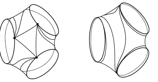
each component of $Q$, and “spin” this triangulation around $Q$, arriving at a lamination $\lambda$

whose closed leaves are $Q$ and whose other leaves spiralonto $Q$,

as

in Figure 1.

Auniquepleatedsurface (uptoequivalence) exists carrying$\lambda$togeodesics,

FIGURE 1. The lamination obtained by spinning

a

triangu-lation around a

curve

system. The picture shows

one

pair of pants in

a

decomposition.

observed by Thurston (see [45] and Canary-Epstein-Green [13, Thm 5.3.6]

for

a

proof). The choices of$\lambda$ coming from the finite number of possible

tri-angulations up to isotopy, and the different directions of spiraling, account for all of pleat$(Q, p)$.

4.2. Elementary

moves.

Anelementary move on amaximalcurve system

$P$ is a replacement of a component $\alpha$ of $P$ by $\alpha’$, disjoint from the rest of

$P$, so that $\alpha$ and $\alpha’$

are

in one of the two configurations shown in Figure 2.

FIGURE 2. The two types ofelementary

moves.

We indicate this by $Parrow P’$ where $P’=P\backslash \{\alpha\}\cup\{\alpha’\}$ is the new

curve

system. Note that there

are

infinitelymany choices for $\alpha’$, naturally indexed

by Z.

Pleated surfaces associated to an elementary move

are

homotopic in a controlled way. Let us first recall (see Buser [10]) that a simple geodesic $\gamma$

in a hyperbolic surface $(S, \sigma)$ always admits

a

($‘ \mathrm{s}\mathrm{t}\mathrm{a}\mathrm{n}\mathrm{d}\mathrm{a}\mathrm{r}\mathrm{d}$collar”, whichis an

disjoint collars, and when $\ell_{\sigma}(\gamma)<\epsilon_{0}$ the collar

covers

all but a bounded part

of the $\epsilon_{0}$-Margulis tube. We write this collar as collar$(\gamma, \sigma)$, or collar$(P, \sigma)$

for the union of collars over a curve system $P$.

Lemma 4.1. (Elementary Homotopy)

_If

$P_{0}arrow P_{1}$ is an elementary move exchanging $\alpha_{0}$ and $\alpha_{1},$ $\rho$ is a Kleinian

surface

group, and $f_{i}\in \mathrm{p}\mathrm{l}\mathrm{e}\mathrm{a}\mathrm{t}(P_{i,\rho})$

for

$i=0,1$ , then there exists a homotopy $H$ : $S\mathrm{x}[0,1]arrow N_{\rho}$ with the

following properties:

1. $H_{0}\sim f_{0}$ and $H_{1}\sim f_{1}$ under the usual equivalence.

2.

_If

$\sigma_{i}$ is the induced metric

of

$H_{i}$ (for $i=0,1$) then collar$(P_{j}, \sigma_{i})=$ $\mathrm{c}\mathrm{o}\mathrm{l}\mathrm{l}\mathrm{a}\mathrm{r}(P_{j}, \sigma_{1-i})$,

for

$j=0,1$.

3. The metrics $\sigma_{0}$ and$\sigma_{1}$ are $K$-bilipschiiz except possibly when $l_{\rho}(\alpha_{i})<$

$\epsilon_{0}$

for

$i=0$ or 1. In that case the metrics are locally K-bilipschitz

outside collar$(\alpha_{0})\cup \mathrm{c}\mathrm{o}\mathrm{l}\mathrm{l}\mathrm{a}\mathrm{r}(\alpha_{1})$ (orjust one collar

if

only one curve is

short in $N_{\rho}$).

4. The trajectories $H(p\cross[0,1])$ are bounded in length by $K$ except possibly

when $p\in \mathrm{c}\mathrm{o}\mathrm{l}\mathrm{l}\mathrm{a}\mathrm{r}(\alpha_{i})$ and $\ell_{\rho}(\alpha_{i})<\epsilon_{0}$, in which case they are bounded

outside

_of

$\mathrm{T}_{\rho(\alpha_{i})}$.

The constant $K$ depends only on the genus

of

$S$.

(Note that collar$(\alpha_{i})$ in (3) and (4) makes sense without specifying the

metric $\sigma_{j}$, since the two are equal by (2).)

It is worth pointing out that this theorem applies without any a-priori bounds on the lengths $\ell_{\rho}(P_{i})$. The proof is an application of Thurston’s

Uniform Injectivity theorem for pleated surfaces, and the closely related Efficiency of Pleated Surfaces [44] (see also Canary [12]). These theorems control the amount kind ofbending that can occur in a pleated surface, and in particular

can

be used to compare two pleated surfaces that share part of their pleating locus.

We also remark that part (2) isjust for convenience–it iseasy to arrange by an appropriate isotopy.

4.3. Resolution sequences. In [29], we show the existence of special se-quences of elementary moves that

are

controlled in terms of the geometry of the complex of curves, and particularly the projections $\pi_{Y}$. First

some

terminology: if $P_{0}arrow P_{1}arrow\cdotsarrow P_{n}$ is an elementary-move sequence and

$\beta$ is any simple closed curve, denote

$J_{\beta}=\{i\in[0, n] : \beta\in P_{i}\}$.

(Here $\beta\in P$

means

$\beta$ is acomponent of$P.$) We also denote $J_{\beta_{1},\ldots,\beta_{k}}=\cup J_{\beta_{i}}$.

Note that if $\beta$ is a curve and $J_{\beta}$ is an interval $[k, l]$, then the elementary

move $P_{k-1}arrow P_{k}$ exchanges some $\alpha$ for $\beta$, and _{$P_{l}arrow P_{l+1}$} exchanges $\beta$ for

some $\alpha’$. Both

$\alpha$ and

$\alpha’$ intersect

$\beta$, and we call them the predecessor and

Theorem 4.2. (Controlled Resolution Sequences) Let$P$ and $Q$ be maximal curve systems in S. There exists a geodesic $\beta_{0},$

$\ldots,$$\beta_{m}$ in $C_{1}(S)$ and an

elementary move sequence $P_{0}arrow\ldotsarrow P_{n}$, with the following properties:

1. $\beta_{0}\in P_{0}=P$ and $\beta_{m}\in P_{n}=Q$.

2. Each $P_{i}$ contains some $\beta_{j}$.

3. $J_{\beta}$,

if

nonempty, is always an $interval_{f}$ and

if

$[i, j]\subset[0, m]$ then

$|J_{\beta_{i},\ldots,\beta_{j}}| \leq K(j-i)\sup_{Y}d_{Y}(P, Q)^{a}$,

where the supremum is over only those

_subsurfaces

$Y$ whose boundary curves are components

_of

some $P_{k}$ with $k\in J_{\beta_{i},\ldots,\beta_{j}}$.

4.

_If

$\beta$ is a curve with non-empty $J_{\beta_{2}}$ then its predecessor and successor

curves $\alpha$ and

$\alpha’$ satisfy

$|d_{\beta}(\alpha, \alpha’)-d_{\beta}(P, Q)|\leq\delta$. The constants $K,$$a,$$\delta$ depend only on the genus

of

S. The expression $|J|$

for

an interval $J$ denotes its diameter.

The sequence $\{P_{i}\}$ in this theorem is called a resolution sequence. Such

sequences are constructed in [29] by an inductive procedure: beginning with a geodesic $\{\beta_{i}\}$ in $C_{1}(S)$ joining $P$ to $Q$ (we are describing a geodesic here

as a sequence of vertices where successive ones arejoined by edges), we note that the link of each$\beta_{i}$ is itselfa curve complexforasubsurface. Ineach such

complex we add a new geodesic, and repeat. The final structure can then

be $‘(\mathrm{r}\mathrm{e}\mathrm{s}\mathrm{o}\mathrm{l}\mathrm{v}\mathrm{e}\mathrm{d}$” into

a

sequence ofmaximal

curve

systems. Control of the size

of the construction at each stage is achieved by applying the hyperbolicity theorem of [30].

4.4. Contraction and quasi-convexity. Let $C(S, \rho, L)$ denote the

sub-complex of $C$ spanned by the vertices with _$p$-length at most $L$. We will define a map $\Pi_{p}$ : $C(S)arrow P(C(S, \rho, L_{1}))$, where $\prime \mathrm{p}(X)$ is the power set of

$X$, as follows. For _{$x\in C(S)$}, let $P_{x}$ be the curve system associated to the

smallest simplex containing $x$. We define

$\Pi_{\rho}(x)=\bigcup_{f\in \mathrm{p}\mathrm{l}\mathrm{e}\mathrm{a}\mathrm{t}(P_{x},\rho)}\mathrm{s}\mathrm{h}\mathrm{o}\mathrm{r}\mathrm{t}(\sigma_{f})$.

This map turns out to have coarsely the properties of a closest-point pro-jection to a

convex

subset ofa hyperbolic space.

Lemma 4.3. (Contraction Properties) There are constants $b,$$c>0,$ de-pending only on the genus

_of

$S$, such that

for

any $\rho$ the map $\Pi_{\rho}$ has the

following properties:

1. (Coarse Lipschitz)

_If

$d_{C}(x, y)\leq 1$ then

$\mathrm{d}\mathrm{i}\mathrm{a}\mathrm{m}_{C}(\Pi_{\rho}(x)\cup\Pi_{\rho}(y))\leq b$.

2. (Coarse idempotence)

If

$x\in C(S, \rho, L_{1})$ then

3. (Contraction)

_If

$r=d_{C}(x, \Pi_{\rho}(x))$ then

$\mathrm{d}\mathrm{i}\mathrm{a}\mathrm{m}_{C}\Pi_{\rho}(B(x, cr))\leq b$.

Here $d_{C}$ and $\mathrm{d}\mathrm{i}\mathrm{a}\mathrm{m}_{C}$ refer to distance and diameter measured in $C(S)$, and

$B(x, s)$ is a ball of $d_{C}$-radius $s$ around $x$. By $\Pi_{\rho}(X)$ for a set $X$ we

mean

$\bigcup_{x\in X}\Pi_{\rho}(x)$.

Compare this with the contraction property in [30], which was used to prove hyperbolicity of $C(S)$, and the property in [38], which was used to

prove stability properties for certain geodesics in Teichm\"uller space.

An easy consequence of this theorem is the following quasiconvexity

prop-erty for $C(S, \rho, L_{1})$:

Lemma 4.4. (Quasiconvexity)

_If

$\beta_{0},$

$\ldots,$$\beta_{m}$ is a geodesic in $C_{1}(S)$ and

$\beta_{0},$$\beta_{m}\in C(S, \rho, L_{1})$, then

$d_{C}(\beta_{i}, \Pi_{\rho}(\beta_{i}))\leq C$

for

all $i\in[0, m]$ and a constant $C$ depending only on the genus

of

$S$.

In particular a geodesic with endpoints in $C(S, \rho, L_{1})$ never strays too far

from $C(S, \rho, L_{1})$. This

can

be compared to the “Connectivity” lemma in

[39].

The argument for this lemma is very simple, and has its origins in the stability of quasi-geodesics argument in the proof of Mostow’s Rigidity The-orem [41]: We compare the path $\{\beta_{i}\}$ to its image “quasi-path” $\{\Pi_{\rho}(\beta_{i})\}$.

If the distance between these grows too much then the images slow down because of the Contraction property (3). Since $\{\beta_{i}\}$ is a shortest path and

the two paths have nearly the same endpoints (Coarse idempotence (2)),

there is a bound on how far apart they

can

get.

The proof of Lemma 4.3 is another application of Thurston’s Uniform Injectivity theorem, as well

as

some of the tools developed in [30]. For example, to prove part (1),

we

note that if two vertices of $C(S)$

are

at

distance 1 then they correspond to disjoint curves, and hence

a

pleated surface exists that maps both geodesically. Thus the argument reduces to bounding $\Pi_{\rho}(x)$ for

one

$x$. Suppose two pleated surfaces share

a curve

$x$. If $x$ is short then their short curve sets intersect, and we finish by noting that

$\mathrm{d}\mathrm{i}\mathrm{a}\mathrm{m}_{C}$(short$(\sigma)$) is uniformly bounded for any $\sigma$. If the curve $x$ is long, then in one of the pleated surfaces we can find a curve $x’$ of bounded length that

runs

along $x$ and then makes a very small jump in its complement

(a long

curve

in a hyperbolic surface must run very close to itself). The

Uniform Injectivity theorem is then applied to show that $x’$

can

be realized with bounded length on the second pleated surface as well.

Part (3) is the main point of the lemma. Its proof dependson the analysis in [30], which shows roughly that if$x\in C(S)$ is far in $C(S)$ from the short

curves

of a given hyperbolic metric $\sigma$

on

$S$, then sets of the form $B(x, R)$

for large $R$ can be carried in a long nested chain of “train tracks” (see [43])

used to control $\Pi_{\rho}(B(x, R))$, via a Uniform Injectivity argument similar to

the previous paragraph.

4.5. Building a resolution sequence for $\rho$

.

We can now use Theorem

4.2 (Controlled Resolution Sequences) and Lemma 4.4 (Quasiconvexity) to

producearesolution sequenceadapted to the geometry of

our

representation

$\rho$.

As a starting point we need an initial and terminal curve system:

Lemma 4.5. Given $\rho$ with

no

externally short curves, and a Margulis tube $\mathrm{T}_{\gamma}$ in $N_{\rho}$, there exist maximal curve systems $P_{+}$ and $P_{-}$, and pleated

sur-faces

$f_{+},$ $f_{-}$ (in the homotopy class

of

$\rho$) with the following properties:

1. $P_{\pm}\in \mathrm{s}\mathrm{h}\mathrm{o}\mathrm{r}\mathrm{t}(\sigma_{f\pm})$,

2. $f_{+}$ and $f$-homologically encase $\mathrm{T}_{\gamma}$.

This is done roughly as follows. If$\nu_{+}$ is a lamination then there exists a

sequence $g_{i}$ of pleated surfaces exiting the end of $N_{\rho}$ corresponding to $\nu_{+}$.

The

curves

in short$(\sigma_{\mathit{9}i})$

converge

to $\iota/+\mathrm{i}\mathrm{n}$the space oflaminations (modulo

measure), and for large enough $i,$ $g_{i}$ can be deformed to $e_{+}$ without meeting

$\mathrm{T}_{\gamma}$. We can pick $f_{+}=g_{i}$ and let $P_{+}\in$ short$(\sigma_{\mathit{9}i})$. The same goes for

$f_{-},$$P_{-}$, so if both invariants are laminations we have the conclusion that $f_{+}$

and $f$-must encase $\mathrm{T}_{\gamma}$.

If the end $e_{+}$ is geometrically finite we

can

let $f_{+}$ be the pleated map to

the

convex

hull boundary itself, and similarly for $e_{-}$. Again choose $P_{\pm}\in$

$\mathrm{s}\mathrm{h}\mathrm{o}\mathrm{r}\mathrm{t}(\sigma_{f\pm})=\mathrm{s}\mathrm{h}\mathrm{o}\mathrm{r}\mathrm{t}(\iota/’\pm)$.

Note that, if the pleated surfaces $g_{i}$ are chosen far enough out the end

(in the geometrically infinite case) then the homotopy from $g_{i}$ to a map

in pleat$(P_{+}, \rho)$ does not pass through $\mathrm{T}_{\gamma}$, and so we may assume $f_{\pm}\in$

$\mathrm{p}\mathrm{l}\mathrm{e}\mathrm{a}\mathrm{t}(P_{\pm,\rho})$ and still have the encasing condition. When there

are

geomet-rically finite ends this is trickier because $\mathrm{T}_{\gamma}$ may be close to the convex

hull boundary. Slightly more

care

is needed in the rest of the construction in that

case.

Let us from

now on assume

that $f_{\pm}\in \mathrm{p}\mathrm{l}\mathrm{e}\mathrm{a}\mathrm{t}(P_{\pm,\rho})$, and the

encasing condition holds.

Join $P_{+}$ to $P$-with a resolution sequence _{$P_{-}=P_{0}arrow\cdotsarrow P_{n}=P_{+}$}, as

in Theorem 4.2. Let $\{\beta_{i}\}_{i=0}^{m}$ be the associated geodesic. This sequence may

be much longer than

we

need,

so we

will

use

Lemma 4.4 to find a suitable subsequence. Recall that

we

would like

our

sequence to have the property of homologically encasing $\mathrm{T}_{\gamma}$,

so

let us try to throw away those surfaces that

we are sure

cannot meet $\mathrm{T}_{\gamma}$. In particular, let $f\in \mathrm{p}\mathrm{l}\mathrm{e}\mathrm{a}\mathrm{t}(P_{i,\rho})$ for some

$i\in[0, n]$, and let $P_{i}$ contain a curve $\beta_{j}$. If $f(S)\cap \mathrm{T}_{\gamma}\neq\emptyset$, then $\gamma$ itself is

short in $\sigma_{f}$ (as in

\S 2.1)

and so $\gamma$ is distance 1 from $\square _{p}(\beta_{j})$. It follows from

Lemma 4.4 that

$d_{C}(\beta_{j,\gamma})\leq C$ $(*)$

where $C$ is a new constant depending only on the genus of $S$. Thus we conclude that there is

a

subinterval $I_{\gamma}$ of $[0, m]$ of diameter at most $2C$,

such that $f$

can

only meet $\mathrm{T}_{\gamma}$ when $\beta_{j}$ satisfies $j\in I_{\gamma}$. Let us therefore restrict our elementary move sequence to

$P_{s-1}arrow\cdotsarrow P_{t+1}$

where $[s, t]= \bigcup_{j\in I_{\gamma}}J_{\beta_{j}}$, and renumber it as $P_{0}arrow\cdotsarrow P_{M}$. This

subse-quence must also

encase

$\mathrm{T}_{\gamma}$, since

none

of the pieces

we

have thrown away

can meet $\mathrm{T}_{\gamma}$. Part (3) of Theorem 4.2 tells us that

$M \leq K(2C)\sup_{Y}d_{Y}(P_{+}, P_{-})^{a}$,

where the supremum is over subsurfaces $Y$ whose boundaries appear among the $P_{i}$ in

our

subsequence. This

means

by _$(*)$ that the $C(S)$-distance $d_{C}(\partial Y, \gamma)$ is bounded by $C+1$ for all such $Y$. The analysis of [29] shows that, for a fixed such bound,

$d_{Y}(P_{+}, P_{-})\leq d_{Y}(\nu_{+}, \nu_{-})+\delta$

with $\delta$ depending only on the genus of _$S$,

provided, when $e_{+}$ or $e_{-}$ are

geometrically infinite, that the surface $f_{\pm}$ are takensufficiently far out in the

ends (for geometrically finite ends this is an easier consequence ofSullivan’s theorem comparing $\nu\pm \mathrm{w}\mathrm{i}\mathrm{t}\mathrm{h}\nu_{\pm}’$, though here we must take a bit

more care

with the constants to make sure that $\partial Y$ intersects _{$P_{\pm}$}). Sincethe right side

is a priori bounded by hypothesis, we obtain our desired uniform bound on

$M$.

Now let $H$ : _{$S\cross[i, i+1]arrow N_{p}$} be the homotopy provided by Lemma 4.1

(Elementary Homotopy), where $H_{i}\in \mathrm{p}\mathrm{l}\mathrm{e}\mathrm{a}\mathrm{t}(P_{i\rho},)$. After possibly adjusting

by homeomorphisms of $S$ homotopic to the identity, we

can

piece these together to a map $H:S\cross[0, M]arrow N_{p}$.

Assume first that $\gamma$ is not a component of any $P_{i}$. Then according to

Lemma 4.1, $H$ can make only uniformly bounded progress through the

Mar-gulis tube $\mathrm{T}_{\gamma}$. Thus diam$\mathrm{T}_{\gamma}$ is bounded above, and $p_{p}(\gamma)$ is bounded below,

and we are done.

Now suppose that $\gamma$ does appear in the $\{P_{i}\}$. Then $J_{\gamma}$ is

some

subinterval

of $[0, M]$ by Theorem 4.2, and

we

let $\alpha$ and $\alpha’$ be the predecessor and

successor curves

to $\gamma$ in the sequence. Both of them

cross

$\gamma$, and we have

by part (4) of Theorem 4.2 that $d_{\gamma}(\alpha, \alpha’)$ is uniformly approximated by

$d_{\gamma}(P_{+}, P_{-})$ and hence uniformly bounded.

For simplicity, let us consider now the case that both $\ell_{\rho}(\alpha)$ and $\ell_{\rho}(\alpha’)$

are uniformly bounded above and below. (There is in fact a uniform upper boundon their lengths; if they become too shortasmall additional argument

is needed).

Let $\sigma_{i}\equiv\sigma_{H_{i}}$ and note that, by Lemma 4.1, for all $i\in J_{\gamma}$ the annuli collar$(\gamma, \sigma_{i})$ coincide. Name this

common

annulus $B$. Write $J_{\gamma}=[k, l]$, and consider in $S\cross[0, M]$ the solid torus

$U=B\cross[k-1, l+1]$.

By Lemma 4.1, this is the only part of $S\cross[0, M]$ that $H$ can map more

is at most $M$ and this is uniformly bounded. The top and bottom annuli

$B\cross\{k-1\}$ and $B\cross\{l+1\}$ have uniformly bounded geometry (in $\sigma_{k-1}$ and $\sigma_{l+1}$, respectively), by the length bounds

$\mathrm{w}\mathrm{e}’ \mathrm{v}\mathrm{e}$ assumed on $\alpha$ and

$\alpha’$. We

will control the size of the meridian of $U$, and this will in turn bound the size of $\mathrm{T}_{\gamma}$.

Assume $\alpha$ is a geodesic in $\sigma_{k-1}$ (where we note its length is bounded

above), and let $a=\alpha\cap B$. Similarly

assume

$\alpha’$ is a geodesic in

$\sigma_{l+1}$ and

let $a’=\alpha’\cap B$_. The arc $a$ may a priori be long in $\sigma_{l+1}$, but its length is

estimated by the number of times it twists around $a’$, or _{$d_{A(B)}(a, a’)$}. A lemma in 2 dimensional hyperbolic geometry establishes

$|d_{A(B)}(a, a’)-d_{\gamma}(\alpha, \alpha’)|\leq C$

where this $C$ depends only on $M$, whichwe have already bounded uniformly.

The idea of this is that, in each elementary move, the metric $\sigma_{i}$ changes in

a bilipchitz way outside the collars of the curves involved in the elementary move. From this it follows that,

start\’ing

with a geodesic passing through a collar, we obtain a curve which does only a bounded amount of additional

twisting,

outside the collar. After $M$ such moves the relative twisting of $\alpha$

and $\alpha’$ can still be estimated by their twisting inside the collar, up to an

additive bound proportional to $M$.

With this estimate and the boundon $d_{\gamma}(\alpha, \alpha’)$ in terms of$d_{\gamma}(P_{+}, P-)$, we find that $a$ and $a’$ intersect a bounded number of times, so that the length

of $a$ is uniformly bounded in $S\cross\{l+1\}$. It follows that the meridian of $U$

$m=\partial(a\cross[k-1, l+1])$

has uniformly bounded length in the induced melric. Thus its image is bounded in $N_{\rho}$. It therefore spans a disk of bounded diameter, and in fact

we can homotope $H$ on all of $U$ to a new map of bounded diameter. This bounds the diameter of $\mathrm{T}_{\gamma}$ from above, and again we are done.

5. CONJECTURES

5.1. Lengthestimates. The readermay have noticed that infact the argu-ment outlined in the previous section shows that the infimum $\epsilon=\inf_{\gamma}\ell_{\rho}(\gamma)$

and the supremum $D= \sup_{Y}d_{Y}(\nu_{+}, \nu_{-})$ can be bounded one in terms of

the other. That is, any positive lower bound for $\epsilon$ implies some upper bound

for $D$ independent of $\rho$, and vice

versa.

Thus there is a version of the

theo-rem which yields non-empty information for quasi-Fuchsian groups (where

$\epsilon>0$ and $D<\infty$ automatically)

as

well. However it would be nice to have

bounds that are more specific and

more

explicit.

“More specific”

means

that

we

would like to know

an

estimate on $p_{p}(\gamma)$

for a particular $\gamma$. In [40] we actually show that for any subsurface $Y$, a

large lower bound on $d_{Y}(u_{+}, \iota/-)$ implies a small upper bound for $\ell_{\rho}(\partial Y)$.

In the other direction something more complicatedwould need to be stated,

“More explicit” means we would like to know the estimate itself

more

explicitly. Furthermore it would be nice to estimate the complex translation length $\lambda$ and not just its real part $\ell$. In [39] this was done for the

punctured-torus case. Here is a possible generalization, stated again in the case of $\rho$

with no externally short curves.

Conjecture 5.1. Let$\rho$ be a Kleinian

surface

group with no externally short

curves. There exist $K,$$\epsilon>0$ depending only on the genus

of

$S$ such that

$\ell_{\rho}(\gamma)>\epsilon\Rightarrow\sup_{\gamma\subset Y}d_{Y}(\iota/+, \nu_{-})<K$. Conversely,

_if

$\sup_{Y}d_{Y}(\nu_{+}, \nu_{-})\geq K$ then

$\frac{2\pi i}{\lambda_{\rho}(\gamma)}\wedge\vee d_{\gamma}(\nu_{+}, \nu_{-})+i\tilde{\sum_{Y\subset S}}d_{Y}(\iota\nearrow_{+},$$\nu_{-)}$

$\gamma\subset\partial YY\not\simeq\gamma$

Let

us

explain the notation used here. The expression $\tilde{\sum_{x\in X}}f(x)$ denotes

$1+$

$\sum_{x\in X,f(x)\geq K}f(x)$

where $K$ is our a-priori “threshold” constant. Our sum then is over all

subsurfaces whose boundary contains the isotopy class of $\gamma$, except for the

annulus homotopic to$\gamma$, excluding those where $d_{Y}(\nu_{+}, \nu_{-})$ is below$K$. Both

sides of the (

$\zeta_{\vee,\wedge}$” symbolare points in the upper halfplaneof$\mathrm{C}$, and we take

$‘\zeta_{\vee}-,$, to mean that the hyperbolic distance between them is bounded by an

a-priori constant $D_{0}$. Implicit in the statement is that it holds for some $D_{0}$

which depends only

on

the genus of $S$.

The significance of the hyperbolic distance estimate on $2\pi i/\lambda(\gamma)$ is that we can interpret $2\pi i/\lambda(\gamma)$

as a

Teichm\"uller parameter for the Margulis tube

$\mathrm{T}_{\gamma}$, as follows (cf. [39] and $\mathrm{M}\mathrm{c}\mathrm{M}\mathrm{u}\mathrm{l}\mathrm{l}\mathrm{e}\mathrm{n}[31]$). Normalize $\rho(\gamma)$ so that it acts

on $\hat{\mathrm{C}}$

by $z-+e^{\lambda}z$. The quotient $(\mathrm{C}\backslash \{0\})/\rho(\gamma)$ is then a torus, and there is a preferred marking of this torus by the pair $(\hat{\gamma}, \mu)$, where

$\mu$ is the meridian

of the torus, or the image of the unit circle in $\mathrm{C}$, and

$\hat{\gamma}$ is the image of

the curve $\{e^{t\lambda} : t\in[0,1]\}$

.

Note, this curve depends on the choice of $\lambda$

mod $2\pi i$. In [39]

we

point out that if$p_{\rho}(\gamma)$ is sufficiently short then

we can

choose $\hat{\gamma}$ to be

a

minimal representative of

$\gamma$

on

the torus just by choosing

$\theta={\rm Im}\lambda\in[0,2\pi)$.

The quantity $2\pi i/\lambda$ turns out to be the point in the upper half-plane

representation of the Teichm\"uller space of the torus which represents the marked quotient torus. Estimating this quantity up to bounded hyperbolic distance is then equivalent to estimating the torus structure up to bounded

Teichm\"uller distance, which corresponds to knowing the action of$\rho(\gamma)$ up to

bilipchitz conjugacy of the action

on

$\mathrm{H}^{3}$, and thus is the “right” kind of

esti-mate ifwe

are

interested in knowing the quotient geometry up to bilipschitz equivalence.

The imaginary part of the conjectural estimate is supposed to estimate the “height” of the margulis tube boundary for $\gamma$, and its real part is

sup-posed to

measure

the $‘(\mathrm{t}\mathrm{w}\mathrm{i}\mathrm{s}\mathrm{t}$” of the meridian around $\hat{\gamma}$. In our discussion of

the Bounded Geometry Theorem, we essentially showed that the height

was

bounded by the number of elementary

moves

it took to pass $\mathrm{T}_{\gamma}$, and the

twisting was bounded by the relative twisting of the predecessor and suc-cessor curves $\alpha$ and

$\alpha’$. In general we expect that large values of

$d_{Y}(\nu_{+}, u_{-})$ with $\gamma\subset\partial Y$ will contribute to parts of the elementary move sequence that

make progress along the sides of $\mathrm{T}_{\gamma}$, and thus give a good estimate for its

height.

In [39] we obtained a similar estimate for the

case

where $S$ is a once-punctured torus. (In this case we are not requiring $S$ to be closed, and our representations must satisfy the added condition that the conjugacy class corresponding to loops around the puncture is mapped to parabolics.) Let us state this just in the case that $\nu\pm \mathrm{a}\mathrm{r}\mathrm{e}$ both laminations. For the torus, a

lamination

are

determined by its slope in$H_{1}(S, \mathrm{R})=\mathrm{R}^{2}$, which takes values in $\hat{\mathrm{R}}=\mathrm{R}\cup\{\infty\}$. Simple closed

curves

correspond to rational points. For

any simple closed curve $\alpha$ we defined a quantity analogous to $d_{\alpha}(\nu_{-}, \nu_{+})$ as

follows: after an appropriate basis change for $S$ (or equivalently action by an element of $\mathrm{S}\mathrm{L}_{2}(\mathrm{Z})$, we may

assume

that $\alpha$ is represented by $\infty$, and let $\nu_{-}(\alpha),$ $\nu_{+}(\alpha)$ be the irrational numbers representing the ending laminations.

Then define

$w(\alpha)=\nu_{+}(\alpha)-\nu_{-}(\alpha)$.

We showed that $\ell_{p}(\alpha)$ canonlybe short if$w(\alpha)$ is above auniform threshold, and in this case we estimated

$\frac{2\pi i}{\lambda_{p}(\alpha)}\wedge-w(\alpha)+i$.

In fact $w(\alpha)$ is just a measure of relative twisting of $\nu$-and $\nu_{+}$ around

$\alpha$, and it is not hard to

see

that $|w(\alpha)|$ is estimated by

our

$d_{\alpha}(\nu_{-}, \nu_{+})$,

up to a uniform additive

error.

Thus, this is really the same estimate as in Conjecture 5.1, since there are no essential subsurfaces in $S$ other than annuli.

5.2. General representations. All the methods that we have presented here depend heavily onthe assumption that $\rho$is both faithful and discrete. It

can

be argued, however, that

a

full understanding of the deformation space of hyperbolic structures on

a

manifold would require some better geometric description of the whole representation variety, including indiscrete or

non-faithful points, and it is tempting to try to enlist the complex of curves for this purpose.

The only results I know that offer any hope are in a paper of Bowditch [8], in which he studies general representations for the once-punctured torus

(again with the parabolicity condition for the puncture). Such

a

represen-tation determines a $\mathrm{t}\mathrm{r}\mathrm{a}\mathrm{c}\mathrm{e}$ (closely related to complex translation length) for

every conjugacy class, and in particular for the simple closed curves, which in this case correspond to $\mathrm{Q}\cup\{\infty\}$, viewed as the vertices of the Farey

tesselation of the disk. To every triangle and adjacent pair of triangles is associated a relation among the traces of the vertices, coming from the standard trace identities in $\mathrm{S}\mathrm{L}_{2}(\mathrm{C})$

.

Bowditch uses these relations alone,

without discreteness, to analyze the global properties of the trace function, in particular obtaining a connectedness property for sublevel sets closely analogous to the quasi-convexity property of Lemma 4.4. Using this he is able to define

an

invariant of the representation that generalizes the ending lamination for discrete representations; but it is hard to know how to extract more information from this invariant.

In the higher genus case, no such analysis has been done, and it would be very interesting to try it. Elementary

moves

between pants decompositions

stillgive rise to trace identities amongthe curves involved, although theyare a bit

more

complicated. One wonders at least whether a result like Lemma 4.4 can be generalized to all representations.

Bowditch is led to the following question: Consider the quantity

$\frac{\ell_{\rho}(\gamma)}{\ell_{\rho_{0}}(\gamma)}$

where$\rho_{0}$ is somefixed Fuchsian representation, $\rho$ is ageneral representation,

and $\gamma$ is a non-trivial element of$\pi_{1}(S)$. The infimum of this ratio is positive

for quasi-Fuchsian representations. For a non-quasi-Fuchsian discrete, faith-ful representation, the infimum is$0$, and can be achieved byconsidering only

$\gamma$ with simple representatives. The limit points of minimizing sequences in

the space of laminations give the ending laminations for $\rho$.

If$\rho$ is indiscrete or non-faithful the infimum is again $0$ (indeed inf$\ell_{\rho}$ is $0$

as well), but the question is, is the infimum also $0$ for the simple elements.

In other words:

Question 5.2. Let $S$ be a closed

surface

of

genus at least 2, and let let

$\rho$ : $\pi_{1}(S)arrow PSL_{2}(\mathrm{C})$ be a representation.

If

$\inf\frac{\ell_{\rho}(\gamma)}{\ell_{\beta 0}(\gamma)}>0$

where $\gamma$ varies over all simple loops in $S$, must $\rho$ be quasi-Fuchsian $‘.p$

This question appears to be difficult, and a positive answer would be a good starting point in using the complex of

curves

to analyze general representations. To indicate its difficulty, note that it is closely related to the following:

Question 5.3.

_If

$\rho$ : $\pi_{1}(S)arrow PSL_{2}(\mathrm{C})$ is any representation with

A positive

answer

to this question is at least as hardto prove

as

the simple loop conjecture for hyperbolic 3-manifolds; see Gabai [17] and Hass [21].

REFERENCES

1. R. Benedetti and C. Petronio, Lectures on hyperbolic geometry, Springer-Verlag Uni-versitext, 1992.

2. L. Bers, On boundaries _ofTeichm\"ullerspaces and on Kleiniangroups I, Ann. of Math.

91 (1970), 570-600.

3. –, Spaces ofdegenerating Riemann surfaces, Discontinuousgroups andRiemann

surfaces, Ann. of Math. Stud. 79, Princeton Univ. Press, 1974, pp. 43-59.

4. Lipman Bers, An inequality_for Riemann surfaces, Differential geometry andcomplex

analysis, Springer, Berlin, 1985, pp. 87-93.

5. F. Bonahon, Closed curves on surfaces, monograph in preparation.

6. –, Geodesic laminations on surfaces, to appear in Proceedings of the Stony

Brook 1998 Workshop on Foliations andLaminations.

7. –, Bouts des vari\’et\’es hyperboliques de dimension 3, Ann. ofMath. 124 (1986), 71-158.

8. B. H. Bowditch, _Markofftriples and quasi-Fuchsian groups, Proc. London Math. Soc.

(3) 77 (1998), no. 3, 697-736.

9. R. Brooks and J. P. Matelski, Collars in Kleinian groups, Duke Math. J. 49 (1982),

no. 1, 163-182.

10. P. Buser, Geometry and Spectra _of Compact Riemann Surfaces, Birkh\"auser, 1992.

11. R. Canary, M. Culler, S. Hersonsky, and P. Shalen, Density _ofcusps in boundaries _of quasiconformal _deformation spaces, in preparation.

12. R. D. Canary, Algebraic limits _ofschottkygroups, Trans. Amer. Math. Soc. 337(1993),

235-258.

13. R. D. Canary, D. B. A. Epstein, and P. Green, Notes on notes _of Thurston,

Analyt-ical and Geometric Aspects of Hyperbolic Space, Cambridge University Press, 1987,

London Math. Soc. Lecture Notes Series no. 111, pp. 3-92.

14. A. J. $\dot{\mathrm{C}}$

asson andS. A. Bleiler, Automorphisms _{of surfaces after}Nielsen and Thurston,

Cambridge University Press, 1988.

15. D. B. A. Epstein andA. Marden, Convexhulls in hyperbolic space, a theorem _of

Sulli-van, and measured pleated surfaces, Analytical and Geometric Aspects ofHyperbolic

Space, Cambridge University Press, 1987, London Math. Soc. Lecture Notes Series no. 111, pp. 113-254.

16. B. Farb, A.Lubotzky, andY. $\mathrm{M}\mathrm{i}\mathrm{n}\dot{\mathrm{s}}\mathrm{k}\mathrm{y}$

, Rank onephenomena_formapping class groups,

preprint.

17. David Gabai, The simple loop conjecture, J. Differential Geom. 21 (1985), no. 1, 143-149.

18. J. Harer, Stability_ofthe homology_ofthe mapping class group _ofan orientable surface,

Ann. of Math. 121 (1985), 215-249.

19. –, The virtual cohomological dimension of the mapping class group of an

ori-entable surface, Invent. Math. 84 (1986), 157-176.

20. W. J. Harvey, Boundary structure _ofthe modular group, RiemannSurfaces and Related Topics: Proceedings of the 1978Stony Brook Conference (I. Kra and B. Maskit, eds.),

Ann. of Math. Stud. 97, Princeton, 1981.

21. Joel Hass, Minimal _surfaces in _manifolds with $S^{1}$ actions and the simple loop

conjec-ture_{for Seifert fibered} spaces, Proc. Amer. Math. Soc. 99 (1987), no. 2, 383-388.

22. A. E. Hatcher andW. P. Thurston, Apresentation_forthe mapping classgroup,

Topol-ogy 19 (1980), 221-237.

23. N. V. Ivanov, Complexes _ofcurves and the Teichm\"uller modular group, Uspekhi Mat.

24. N. V.Ivanov, The rank _ofTeichm\"ullermodulargroups, Mat. Zametki 44 (1988), no. 5, 636-644, 701, translation in Math. Notes 44 (1988), no. 5-6, 829-832.

25. N. V. Ivanov, Complexes _of curves and Teichm\"uller _{spaces, Math. Notes 49} (1991),

479-484.

26. N. V. Ivanov, Subgroups _of Teichm\"uller modulargroups, American Mathematical

So-ciety, Providence, RI, 1992, translated from the Russian by E. J. F. Primrose and

revised by the author.

27. N. V. Ivanov, Automorphisms _of complexes _of curves and _of Teichm\"uller spaces,

In-ternat. Math. Res. Notices (1997), no. 14, 651-666.

28. D. Kazhdan and G. Margulis, A proof _of Selberg’s conjecture, Math. USSR Sb. 4

(1968), 147-152.

29. H. A. Masur and Y. Minsky, Geometry _ofthe complex_ofcurves II..Hierarchical struc-ture, $\mathrm{E}$-printmath._{$\mathrm{G}\mathrm{T}/9807150$} athttp:$//\mathrm{f}\mathrm{r}\mathrm{o}\mathrm{n}\mathrm{t}.\mathrm{m}\mathrm{a}\mathrm{t}\mathrm{h}.\mathrm{u}\mathrm{c}\mathrm{d}\mathrm{a}\mathrm{v}\mathrm{i}\mathrm{s}.\mathrm{e}\mathrm{d}\mathrm{u}$ .To appear inGeom.

Funct. Anal.

30. –, Geometry ofthe complexofcurvesI: Hyperbolicity,Invent. Math. 138 (1999), 103-149.

31. C. McMullen, Cusps are dense, Ann. of Math. 133 (1991), 217-247.

32. R. Meyerhoff, A lower bound _for the volume _of hyperbolic 3-manifolds., Canad. J. Math. 39 (1987), 1038-1056.

33. Y. Minsky, Bounded geometry in Kleinian groups, in preparation.

34. –, Teichm\"uller geodesics and ends of hyperbolic 3-manifolds, Topology 32

(1993), 625-647.

35. –, On rigidity, limit sets and end invariants ofhyperbolic 3-manifolds, J. Amer.

Math. Soc. 7 (1994), 539-588.

36. –, On Thurston’s ending lamination conjecture, Proceedings of Low-Dimensional

Topology, May 18-23, 1992, International Press, 1994.

37. –, A geometric approach to the complex of curves, Proceedings of the 37th

Taniguchi Symposium on Topology and Teichm\"uller Spaces (S. Kojima et. al., ed.),

World Scientific, 1996, pp. 149-158.

38. –, Quasi-projections in Teichm\"uller space, J. Reine Angew. Math. 473 (1996), 121-136.

39. –, The classification ofpunctured-torus groups, Annals of Math. 149 (1999), 559-626.

40. –, Kleiniangroups and the complexofcurves, Geometry and Topology 4 (2000),

117-148.

41. G. D. Mostow, Quasiconformal mappings in $n$-space and the rigidity of hyperbolic

space forms, Publ. I.H.E.S. 34 (1968), 53-104.

42. K. Ohshika, Ending laminations and boundaries _{for deformation} spaces _ofKleinian

groups, J. London Math. Soc. 42 (1990), 111-121.

43. R. Penner and J. Harer, Combinatorics oftrain tracks, Annals of Math. Studies no.

125, Princeton University Press, 1992.

44. W. Thurston, Hyperbolic structures on 3-manifolds, II.. _surface groups

and _manifolds which _fiber over the circle, $\mathrm{E}$-print: math.

$\mathrm{G}\mathrm{T}/9801045$ at

http:$//\mathrm{f}\mathrm{r}\mathrm{o}\mathrm{n}\mathrm{t}.\mathrm{m}\mathrm{a}\mathrm{t}\mathrm{h}.\mathrm{u}\mathrm{c}\mathrm{d}\mathrm{a}\mathrm{v}\mathrm{i}\mathrm{s}.\mathrm{e}\mathrm{d}\mathrm{u}$. Original 1986.

45. –, The geometry and topology of 3-manifolds, Princeton University Lecture

Notes, online at http:$//\mathrm{w}\mathrm{w}\mathrm{w}.\mathrm{m}\mathrm{s}\mathrm{r}\mathrm{i}.\mathrm{o}\mathrm{r}\mathrm{g}/\mathrm{p}\mathrm{u}\mathrm{b}\mathrm{l}\mathrm{i}\mathrm{c}\mathrm{a}\mathrm{t}\mathrm{i}\mathrm{o}\mathrm{n}\mathrm{s}/\mathrm{b}\mathrm{o}\mathrm{o}\mathrm{k}\mathrm{s}/\mathrm{g}\mathrm{t}3\mathrm{m}$, 1982.

46. –, Three-Dimensional Geometry and Topology, Princeton University Press, 1997,

(S. Levy, ed.).