The tensor structure of the original Navier-Stokes equations (Study of the History of Mathematics)

(1)

The

tensor

structure

of the original

Navier-Stokes

equations

SHIGERU MASUDA

Graduate school ofTokyoMetropolitan University, doctoral cource in mathematics E-mail: [email protected]

Abstract

The two-constants theory introduced first by Laplace in 1805 is currently accepted theory describing isotropic, linear elasticity. The original, macroscopically-descriptive Navier-Stokesequations [MDNS

equa-tions]werederivedin thecourseofthe development thetwo-constantstheory. Fromthe viewpoint ofMDNS

equations, we tracetheevolution ofthe equations and the notionof tensor following in historical order the various contributions ofNavier, Cauchy, Poisson, Saint-Venant and Stokesl, and note the concordance be-tween each.

Keywords. the microscopically descriptive equation, the Navier-Stokesequations, mathematicalhistory.

1 Preliminary

Remarks

In this report, we

use

the followingdefinition of the stresstensor, due toI. Imai[7, p.178]:

we

call

a

$P$ of$3\cross 3$

matrix such as $P$ a stress tensor that returns a

new

vector $P_{n}$ when multiplied from the right by the column

vectorof directional cosines :

$\{\begin{array}{l}P_{nx}P_{ny}P_{nz}\end{array}\}=\{\begin{array}{lll}p_{xx} p_{?/x} p_{zx}p_{xy} p_{yy} p_{zy}p_{xz} Pyz p_{zz}\end{array}\}\{\begin{array}{l}lmn\end{array}\}$ $\Rightarrow$ $P_{n}=P\cdot n$

Moreover, if$p_{ij}=p_{ji}$ for all $i.j=x,$$y,$$z$ then this tensor is said to be symmetric. If

we

suppose forexample

$t_{ij}$ is the $(i, j)$ element of amatrix, and $t_{tj}=-t_{ji}$ then anti-symmetric

or

skew-symmetric. Troughout the

paper, we display for brevity a tensor by specifying its components, such

as

$\delta_{ij}$ of the well-known Kronecker $\delta$.

Furthermore, we write $v_{k,k}= \sum_{i=1}^{3}\vec{\partial x}\partial v$

.

$= \frac{du}{dx}+\frac{dv}{dy}+\frac{dw}{dz}\cdots$ where we have the Einstein

convention2.

Simpli-fications

occur

as, for example, in Navier’s elasticity of (1-1) in Table 4 where the tensor can be expressed

as

follows:

$- \epsilon[\{+\frac{d_{?}}{d}++3(\frac{d\iota}{d_{t}}\frac\frac{dc\iota}{dydv,/dyv)}++\frac{du}{(dz}\frac{dv}{dx}\frac{du\{}{dx}\frac{dwdvdx}{dz}\frac++\frac\frac{du}{dz}\}]$

$=- \in[+\frac{dvux}{dudx,dz}2\frac{d}{d}$ $\frac{d}{}+\frac{dy\epsilon dvu}{dz}+\frac{\frac ddd\frac xdvvd^{1/}w}{dy}+2$ $\frac{}{\frac{dwdvdx}{dz\epsilon}}++2\frac{\frac{du}{dwd\tau/dwdzdz}}{}+\frac]$

, (1)

where $\epsilon=\frac{du}{dx}+\frac{dv}{d\tau/}+\frac{dw}{dz}$

Expressions in Poisson’selasticity (3-1) in Table 4

are

also ofsimilar style.

Moreover,

we

can

easily express Navier’s stress tensor$t_{ij}$ ofelasticityin the form: $t_{ig}=-\epsilon(\delta_{ij}u_{k,k}+u_{\iota,j}+u_{j,i})$.

Stokes’ fluid theory (20) or (5) in Table 4 affords a second illustration: $t_{ij}=(-p- \frac{2}{3}\mu?fk,k)\delta_{lJ}+\mu(v_{i,j}+v_{j,i})$,

orthe equivalent expression $\sigma_{ij}=-p\delta_{ij}+\mu(\vec{\partial x_{J}}\partial\tau’+\frac{\partial}{\partial}\lrcorner^{v})-\frac{2}{3}\delta_{ij^{\frac{\partial}{\partial}L}}^{\tau’.3}$ In what follows, ${}^{t}tensor$”means the stress

tensor as defined by I. Imai. 4 _{When referring to} _a _:fluid“, _an _{“elastic fluid’:} _is _implied.

2 Introduction

We have studied the original MDNS equations as the

progenitors5,

Navier, Cauchy, Poisson, Saint-Venant

and Stokes, andendeavor to acertain their aims and conceptual thoughts in formulations these

new

equations.

“The two-constants theory” was introduced first introduced in 1805 by

Laplace6

in regard to capillary action

with constants denoted by $H$ and $K$ (cf. Table 2, 3). Thereafter, various pairsof constants have been proposed

by their originators in formulating MDNS equations

or

equations describing equilibriumorcapillary situations.

It is commonly accepted that this theory describes isotropic, linear

elasticity.7

We argue that Poisson had

already pointed out the special aspect deduced by Laplacewhen, in 1831, he states, ‘elles renferment les deux

constantes sp\’eciales donc$j$’ai parl\’e tout \‘al’heure’ [18, p.4]. Poisson was, wethink, oneof the persons who were

aware

of this issue.

lNavier(1785-1836), Cauchy(1789-1857), Poisson(1781-1840), Saint-Venant(1797-1886), Stokes(1819-1903).

2Remark: in general, $n_{k,k}\neq n_{\iota.j}$, because the summationconvention is in forcewhen thereisarepetition of indices.

$3_{c.f}$. Schlichting [20], in ourfootnote(19).

4Numbers on the Left-hand-side of equations referto those given by the author in the original paper while numberson the

right-hand-side correspond toour indexing. The subscript to the original indexing, for example $N^{e}/N^{f}$, referto author andtype

of theory, such as “elastic/fluid by Navier“. For equations indexed by section, the citation is then in the format “section no.-no. by author“.

5Theorder followedis by date ofproposal or publication.

6Ofcapillaryaction, Laplace[8, V.4, Supplement p.2] achnowledges Clailaut[3, p.22], and Clailautcites Maupertuis[10].

7Darrigol [4. p. 121].

(2)

3 A

universal

method for the

two-constants

theory

Now, we would like to propose the uniformal methods to describe the kinetic equations for isotropic, linear

elasticity

.

such as:

The partial differential equations ofthe elastic solid or elastic fluid areexpressed by using

one

or the pair

of$C_{1}$ and $C_{2}^{Y}$ such that

in the elastic solid: $\frac{\partial^{2}}{\partial t}\tau u-(C_{1}T_{1}+C_{2}T_{2})=f$,

In the elastic fluid: $\frac{\partial u}{\partial t}-(C_{1}T_{1}+C_{2}T_{2})+\cdot\cdot$ $=f$,

where$T_{1},$ $T_{2},$$\cdot$ $\cdot$ aretensorsorterms consistingourequations, wherewesuppose the tensorasthe first kind.

Forexample,the MDNSequationsionscorrespondingto incompressible fluid is composed of the kinetic equation

along with the continuity equation andare conventionally written, in modem vector notation,

as

follows :

$\frac{\partial u}{\partial t}-\mu\triangle u+u\cdot\nabla u+\nabla p=f$, divu_$=0$. (2)

.

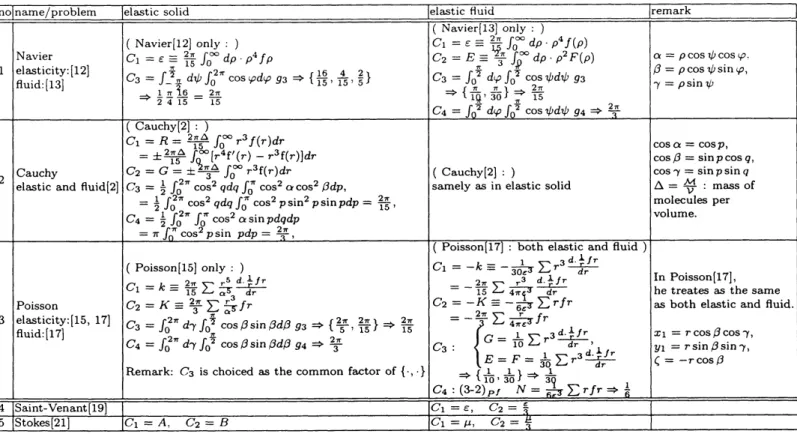
$C_{1}$ and $C_{2}$

are

the two coefficients of the two-constants theory, for example, $\epsilon$ and $E$ by Navier, or $R$ and

$G$ by Cauchy, $k$ and $K$ by Poisson, $\in$ and $\frac{\epsilon}{3}$ by Saint-Venant, or $\mu$ and $\mu 3$ by Stokes. Moreover $C_{1}$ and $C_{2}$

can

be expressed inthefollowing form:

$\{\begin{array}{l}C_{1}\equiv \mathcal{L}r_{1}g_{1}S_{1},\{\end{array}$

$S_{1}= \int\int g_{3}arrow C_{3}$,

$C_{2}\equiv \mathcal{L}r_{2}g_{2}S_{2}$, $S_{2}= \int\int g_{4}arrow C_{4}$,

$\Rightarrow$ $\{\begin{array}{l}C_{1}=C_{3}\mathcal{L}r_{1}g_{1}=\frac{2\pi}{15}\mathcal{L}r_{1}g_{1)}C_{2}=C_{4}\mathcal{L}r_{2}g_{2}=\frac{2\pi}{3}\mathcal{L}r_{2}g_{2}.\end{array}$

.

The two coefficients

are

expressible in terms ofthe operator $\mathcal{L}$

$( \sum_{0}^{\infty}$ or $\int_{0}^{\infty})$ by personal principles or

methods, where$r_{1}$ and $r_{2}$ arethe radialfunctions related to the radius ofthe active sphere of the molecules.

$g_{1}$ and$g_{2}$ are thecertain functions which depend on $r$ and

are

describedwith

attraction&/or

repulsion.

$S_{1}$ and $S_{2}$are thetwo expressions whichdescribe the surface of active unit-sphereatthe center of

a

molecule

by the double integral (or single

sum

in

case

ofPoisson’sfluid).

$g_{3}$ and $g_{4}$

are

certain compound trigonometric functions to calculatethe momentum in the unit sphere.

.

$C_{3}$ and $C_{4}$

are

indirectly determined

as

the

common

coefficients from the invariant tensor. Except for Poisson’s fluid case, $C_{3}$ of$C_{1}$ is $\frac{2\pi}{3}$, and $C_{4}$ of$C_{2}$ is $21F$, which are calculated from the total momentumofthe

activesphere of the molecules in computing only by integral, and which are independent

on

personal manner.

In Poisson’s case, after multiplying by $\frac{1}{4\pi}$, we get the

same as

above.

.

The ratio of the two coefficients including Poisson’s

case

is always

same

as :

_al

$= \frac{1}{5}$.

4 A genealogy and

convergence

of

stress tensor

Weshow in the figure 1, a genealogy tracing in paticular the formofthe tensor $t_{ij}$ appearing in the

Navier-Stokesequations. In Table 4,wedifferentiate the tensors associated with elastic solidsorelasticfluids. $\mathbb{R}om$this

genealogy, it could be asserted that Cauchy[l, 2] wasthe inventor orthefirst

user

of tensors,

a

view supported

by the admissionof Poisson[17] that he received the idea of symmetric tensor from Cauchy. Moreover, the idea

ofSaint-Venant reappearsinthe work ofStokes. Here,wedenotethe two routesas NCP and PSS, both of which

are portrayed in

our

figure, and by which,

we

can explain the genealogy oftensor

as

it applies to the MDNS

equations. cf. Table4.

(fig.1) A genealogy

of

stress tensors inthe prototypical Navier-Stokes equations

Navier $[12||’ 13]J[$ $t_{i_{J}}^{e}\cdot=-\in(\delta_{ij}u_{k,k}+u_{i,j}\backslash +u_{j,i}),$ $t_{zj}^{f}=(p-\in u_{k,k})\delta_{ij}-\in(u_{i,j}+u_{j,i})$ $\nearrow$ $(Euler)\Rightarrow^{\backslash }$ ...

$\Downarrow\Uparrow\Vert Poisson[15,17]$

.

$\Rightarrow^{\nearrow}$

Saint-Venant[19]$\dagger$ $\Rightarrow$ Stokes$[21]\ddagger$

Cauchy[1, 2] : $t_{ij}^{e,f}=\lambda v_{k,k}\delta_{\iota j}+\mu(v_{ij}+v_{ji})$

$\circ$ Poisson : $t_{ij}^{e}=- \frac{a^{2}}{3}(\delta_{ij}u_{k,k}+u_{i,j}+u_{g,i}),$ $t_{ij}^{f}=-p\delta_{ij}+\lambda v_{kk}\delta_{ig}+\mu(v_{i,j}+v_{g,i})$

\dagger Saint-Venant : $t_{ij}^{j}=$ $( \frac{1}{3} (P.. +P_{yy}+P_{zz})-\frac{2\epsilon}{3}v_{k,k})\delta_{ij}+\in(v_{ij}+v_{j,i}),$ $\frac{1}{3}(P_{xx}+P_{yy}+P_{zz})=-p$

\ddagger Stokes: $t_{ij}^{f}=(-p- \frac{2}{3}\mu v_{k,k})\delta_{ij}+\mu(v_{\iota,j}+v_{g,\iota})$,

O Poisson says his reducing of tensor elements to6 from 9is due to Cauchy. (cf.\S 5.2).

5 Deductions of two constants and tensor

Recently Darrigol [4, p.121] has concluded: ‘it is called that thetwo-constantstheoryis the

one now

accepted

for isotropic, linear elasticity,’ but Poisson [18, p.4] has stated already in 1831. ‘elles renferment les deux

constantes sp\’eciales donc $j$’ai parl\’e tout \‘a 1‘heure.’ Moreover,

we

believe that the first proposer of

(3)

Table 1: $C_{1},$$C_{2},$$C_{3)}C_{4}$ the constant of definitions and computing of total momentum of molecular actionsby

(4)

5.1 Navier’s two constants

and

tensor

Inhistheory_{of elasticity, Navier deduced the}_single_constant$\in$in(l). Thecorresponding Navier-Stokesequations

by Navier himself forthe incompressible fluid (2)

are

asfollow :

$\{\begin{array}{l}\frac{1}{\rho}\overline{d}xdp=X+\epsilon(3\frac{d^{2}}{dx}uF+\frac{d^{2}}{dy}ur+\frac{d}{}dz=^{u}2+2\frac{d^{2}v}{dxdy}+2\frac{d^{2}w}{dxdz})-\frac{du}{dt}-\frac{du}{dx}\cdot u-\frac{du}{dy}\cdot v-\frac{du}{dz}\cdot w;\frac{1}{\frac,\rho\rho 1}dR\frac{d}{d}Rz\frac{d}{d}d2xxTw+d^{2}d=^{w}y+3\frac{d^{2}}{dz}\tau w+\frac{d^{2}uxdyd^{2}u}{dxdz}+\frac{d^{2}yw)d^{2}v}{dydz})-\frac{dwvt}{dt}-\frac{dw}{dx}\cdot u-\frac{dw}{dy}v-\frac{dw}{dz}w=^{v}=^{v}d^{2}d^{2}v;\end{array}$

(3)

along with the equationof continuity: $\frac{du}{dx}+\frac{dv}{dy}+\frac{dw}{dz}=0$. Navier supposes two constants

as

follows :

(3-10) $\epsilon\equiv\frac{8\pi}{30}\int_{0}^{\infty}d\rho\rho^{4}f(\rho)=\frac{4\pi}{15}\int_{0}^{\infty}d\rho\rho^{4}f(\rho)$, $E \equiv\frac{4\pi}{6}\int_{0}^{\infty}d\rho\rho^{2}F(\rho)=\frac{2\pi}{3}\int_{0}^{\infty}d\rho\rho^{2}F(\rho)$. (4)

In the

case

of fluid, Navier

was

well

aware

of necessity for the equation of continuity, because from (3) he

obtained $\epsilon\Delta$, by defferentiating the equation

ofcontinuity with $\frac{d}{dx},$$\frac{d}{dy},$$\frac{d}{dz}$. For example, the $\in$-terms in (3),

as

well

as

(5)

are

reduced to $\epsilon\triangle u$ in (6). This is solely due to the mass

conservative law, according to the

explaination given by Navier.

As anaside, _{Navier always used his well-used mathematical methods involving}_a_four-steps_procedure_{to solve}

the three equations such

as

the equilibrium equation for thefluid [13], the kinetic equationfor the elastic [12],

and thekinetic equation forthefluid [13] with the general methods

as

follows:

$\circ$ initially, to deduce

one or

two constants including uncomputable

functions: $g_{1},$ $g_{2}$ i.e. $f\rho,$ $f(\rho)$

or

$F(\rho)$ in

Table 2,

.

then, to construct the indeterminate equation, which he denoted the nomencrature of “equation

undeter-minant” (cf.

.

\S 5.1.1),

then, to make Taylor series expansion and partial integration, exchanging $d$ and $\delta$, and pairing with the

same

.

integral operator,

andfinally, to solve the indeterminateequation from the twopoints ofview, theinterior andthe boundary.

We present

more

details of this procedure by outlining Navier’s analysis of fluid flow[13].

5.1.1 Indeterminate equation

The indeterminate equation, so-called then by Navier, is

as

follows:

(3-24) $f$ $0$ $=$ $\int\int\int dxdydz\{[[Q-\frac{d}{\overline dd}R-\rho\{\begin{array}{l}\frac{du}{dt}+u\frac{du}{dx}+v\frac{du}{dy}+w\frac{du}{dz})]\delta u\frac{dv}{dt}+u\frac{dv}{dx}+v\frac{dv}{dy}+w\frac{dv}{dz})]\delta v\frac{dw}{dt}+u\frac{dw}{dx}+v\frac{dw}{dy}+w\frac{dw}{dz})]\delta w\end{array}$

$-$ $\in\int\int\int dxdydz\{\{\begin{array}{l}3\frac{du}{dx}\frac{\delta du}{dx}+\frac{du}{dy}\frac{\delta du}{dy}+\frac{du}{dz}\frac{\delta du}{dz})+(\frac{dv}{dy}\frac{\delta du}{dx}+\frac{dv}{dx}\frac{\delta du}{dy})+(\frac{dw}{dz}\frac{\delta du}{dx}+\frac{dw}{dx}\frac{\delta du}{dz})\frac{du}{dx}\frac{\delta dv}{dy}+\frac{du}{dy}\frac{\delta dv}{dx})+(\frac{dv}{dx}\frac{\delta dv}{dx}+3\frac{dv}{dy}\frac{\delta dv}{dy}+\frac{dv}{dz}\frac{\delta dv}{dz})+(\frac{dw}{dy}\frac{\delta dv}{dz}+\frac{dw}{dz}\frac{\delta dv}{dy})\frac{du}{dx}\frac{\delta dw}{dz}+\frac{du}{dz}\frac{\delta dw}{dx})+(\frac{dv}{dy}\frac{\delta dw}{dz}+\frac{dv}{dz}\frac{\delta dw}{dy})+(\frac{dw}{dx}\frac{\delta dw}{dx}+\frac{dw}{dy}\frac{\delta dw}{dy}+3\frac{dw}{dz}\frac{\delta dw}{dz})\end{array}$

(5)

5.1.2 Determinated equation operated by Taylor expansion and partial integral

Putting $Sds^{2}E(u\delta u+v\delta v+w\delta w)=0$ of indeterminate equation (5) and performing

a

Taylor series expansion

to first-order and neglecting higher-order terms,

we

get

as

follows:

(3-29) $0=$ $\int\int\int dxdydz\{[[[R_{dz}^{-1}Q_{\overline{d}y}^{d}P_{dx}^{d}--dz_{-\rho}z_{-\rho}-\rho\{\begin{array}{l}\frac{du}{dt}+u\frac{du}{dx}+v\frac{du}{dy}+w\frac{du}{dz})+c(\frac{d}{d}xT2u+\frac{d^{2}}{dy}\tau+d=z)]\delta u\frac{dv}{dt}+u\frac{dv}{dx}+\tau\frac{dv}{dy}+w\frac{dv}{dz})+\in(d^{2}vd^{2}vvdxdy\frac{dw}{dt}+u\frac{dw}{dx}+?)\frac{dw}{dy}+w\frac{dw}{dz})+\epsilon(=+\frac{d}{d}=^{w}2y+=d^{2}dzw)]\delta w\end{array}$ (6)

From (6) we get (3) i.e. the kinetic equationwhich is the firstexpression of(2).

5.1.3 Determinated equation deduced from boundary condition

As the boundary condition, Navier

uses

two constants in

one

equation. In this aspect, his method is the

uniqueamong the original formulators. Navier explains as follows: regardingthe conditions which react at the

points

.

ofthe surface of the fluid. if

we

substitute

$dydz$ $arrow$ $ds^{2}\cos 1$, where

1

: the angles by which the tangent plane makes with the yz-plane

on

the

surface frame,

.

$dxdz$ $arrow$ $ds^{2}\cos m$, where _$m$ : similarly_$m$ is the angles with the xz-plane,

$edxdy$ $arrow$ $ds^{2}\cos n$, where $n$ : samilarly, $n$ is the angles with the xy-plane,

.

$\iint d\tau/dz,$_{$\iint dxdz$}

.

$\iint dxdy$ $arrow$ $Sds^{2}$, where $S$ is the unit normal to the surface at this point,

then becausethefactorsmultiply$\delta u,$$\delta v$and$\delta w$respectivelyreduce to zero,thefollowing determinated equations

should hold for any points of the surface ofthe fluid element:

(3-32) $\{\begin{array}{l}E_{?)}+\epsilon[\cos l(\frac{dxdudu}{dy}Eu+\epsilon[\cos l2\frac+\cos m(\frac{du}{dy}+\frac{d}{2d}+\cos n+\frac{dv}{dx})+\cos m\frac{xv)dv}{dy}+\cos n\}_{\frac+\frac)])}^{\frac{du}{dzdvdz}+\frac{dw}{dwdydx})]=0}=0’Ew+\in[\cos l(\frac{dw}{dx}+\frac{du}{dz})+\cos m(\frac{dw}{dy}+\frac{dv}{dz})+\cos n2\frac{dw}{dz}]=0.\end{array}$ (7)

Here the value of the constant $E$ must vary in accordance with the nature of solid with which the fluid is _in

contact. Theequationsof(7)

are an

expressionofconditions prevailing

on

the boundary condition of the surface

and constitute the so-called boundary conditions. The first terms of the left-hand-side of (7)

are

defined in (4)

for the expressionthat

we

seek for the

sum

of the momenta ofall interactions arising between the molecules

on

the boundary and the fluid, while the second terms

are

the normal derivatives. Here, derivative terms

on

the

left-hand-side of (7) areexpressible

as

$\iota_{i,j}+u_{j,i}$.

5.2 Cauchy’s two

constants

and tensor

(Definition) We suppose that

$a,$ $b,$ $c$: thecoordinate valuesof

a

molecule _$m$in therectanglar

axes

by$x$

.

$y_{\rangle}z;$ $\cdot a+\triangle a,$ $b+\triangle b,$ $c+\triangle c$: the

coordinates of

an

arbitrary molecule $m$ ; $\xi,$ $\eta,$ $\zeta$ : the functions of$a$

.

$b,$ $c$,which representthe infinitesimal

displacements, and are parallel to the

axes

of a molecule $m$ ; $o(x. y, z),$ $(x+\triangle x, y+\triangle y, z+\triangle z)$ : the

coordinates of the molecules $m$ and $m$ in the new stateof the system ;

.

$r(1+\in)$ : the distance between the

molecule $m$ and $m$ ;

.

$\in:$ the dilatation of the length $r$ in the path from the first state to the second, and

then we have $x=a+\xi,$ $y=b+\eta$. $z=c+\zeta$ ;

.

X. $Y,$ $Z$ . the quantities ofthe algebraic projections.

Cauchy deduces the three elements $X,$ $Y,$ $Z$ in the sysytemofmeterial points of elasticity after calculating

the interactions of molecules, the details ofwhich

are

omitted for sake of brevity. Moreover we start with the

following equationofelasticity

(40) $\{\begin{array}{l}X=(L+c)_{\partial}^{\partial}A_{a}^{2}+(R+H)\frac{\partial^{2}}{\partial b}\xi+(Q+I)\frac{\partial^{2}}{\partial c}\xi+2R\frac{\partial^{2}\eta}{\partial a\partial b}+2Q\frac{\partial^{2}\zeta}{\partial c\partial a},Y=(R+G)\frac{\partial}{\partial}a\phi 2+(M+H)\partial\partial 4^{2}b+(P+I)\partial\partial 4^{2}c+2P\frac{\partial^{2}\zeta}{\partial b\partial c}+2R\frac{\partial^{2}\xi}{\partial a\partial b},Z=(Q+G)\frac{\partial^{2}\zeta}{\partial a^{2}}+(P+H)\frac{\partial^{2}\zeta}{\partial b^{2}}+(N+I)\frac{\partial^{2}\zeta}{\partial c^{2}}+2Q\frac{\partial^{2}\xi}{\partial c\partial a}+2P_{b\partial_{C}^{L}}^{2}\frac{\partial}{\partial}\lrcorner\end{array}$

(The invariants of the tensor

are

represented by the twoconstants of$G$ and $R$. )

Cauchy says about the elements oftensor i.e. the invariable values G. H.$I,$$L$,M.$N,$$P,$$Q,$ $R$:

If we suppose that the molecules $m$.$m’,$$m$“, are originally allocated by the

same

way in relation to the

three planes made by the molecule $m$in parallel with the plane coordinates, then the valuesof these quantities

come

to remain invariable, even though aseries ofchanges are made among the three angles : $\alpha.\beta.\gamma$.

Cauchy considers symmetric tensor such that

(6)

(46) $\{_{Z(R+G^{\gamma})}Y==(R+G^{Y})\}_{\frac+\frac+\frac}^{\frac+\frac+\frac\}_{+2R\frac}^{+2R\frac}}+2R\frac{\partial a\partial\nu\partial_{\mathcal{U}}}{\partial\nu,\partial c\partial b}\}$ (47) $\iota\nearrow=\frac{\partial\xi}{\partial a}+\frac{\partial\eta}{\partial b}+\frac{\partial\zeta}{\partial c}$

Cauchymaybe theinventorofthe

nomenclature8

of “tensor“, andPoisson backsup thestructure ofsymmetry

such that his idea reducing from 9 to 6 elements is due to Cauchy,

as

follows :

D’un autre c\^ot\’e, il faut, pour l’equilibre d’un parall\’el\’epip\‘ede rectangle d’une \’etendue insensible, que

les neuf composantes des pressions appliqu\’ees \‘ases trois faces non-parall\’elles, se r\’eduisent \‘asix forces qui peuvent\^etre in\’egales. Cette proposition est due \‘aM.Cauchy, et sed\’eduit de laconsid\’eration desmomens.

[17, \S 38, p.83]

Continuing,

we

define the densityof molecules as: (48)$c$ $\triangle=\frac{\mathcal{M}}{v}$, where, $\Lambda\Lambda$ isthesum ofthe

mass

of molecules

contained inthe sphereandV isthevolume of thesphere. Wethefindexpression forthetwo constants, $G$ and

$R$:

(50)$c$ $\{\begin{array}{l}G=\pm\frac{\Delta}{2}\int_{0}^{\infty}\int_{0}^{2\pi}\int_{0}^{\pi}r^{3}f(r)\cos^{2}\alpha\sin pdrdqdp =\pm\frac{2\pi\Delta}{3}\int_{0}^{\infty}r^{3}f(r)dr,R=\frac{\Delta}{2}\int_{0}^{\infty}\int_{0}^{2\pi}\int_{0}^{\pi}r^{3}f(r)\cos^{2}\alpha\cos^{2}\beta\sin pdrdqdp =\frac{2\pi\triangle}{15}\int_{0}^{\infty}r^{3}f(r)dr=\pm\frac{2\pi\Delta}{15}\int_{0}^{\infty}[r^{4}f’(r)-r^{3}f(r)]dr\end{array}$ (8)

When wecalculate these values in the general

case

then (8) yieldsthe following expressions:

(56) $\{B\equiv C\equiv\{\begin{array}{l}(L+G)_{\delta a}^{\partial\xi}+(R-G)\frac{\partial\eta}{\partial b}+(Q-G)\frac{\partial}{\partial}\leq_{c}]\triangle,(R-H)\frac{\partial}{\partial}4a+(M+H)\frac{\partial\eta}{\partial b}+(P-H)_{\partial c}^{\partial}\Delta]\Delta,(Q-I)\frac{\partial\xi}{\partial a}+(P-I)_{\partial b}^{\partial}\Delta+(N+I)\frac{\partial\zeta}{\partial c}]\Delta,\end{array}$ (57) $\{E\equiv D\equiv F\equiv\ovalbox{\tt\small REJECT}$

$(Q+G)+(Q+I)_{\partial c}^{\partial}(P+I) \frac{\partial\eta}{\partial c,\Delta\partial a\partial}+(P+H)_{\partial b}^{\partial}1\Delta f_{\triangle}^{\triangle},$

’

$(R+H)_{\partial b}^{\partial} \angle+(R+G)\frac{\partial\eta}{\partial a}]\Delta$,

$\frac{BA}{\Delta}=2(R+G)_{\check{\partial})}^{t_{a}^{45)_{C},weobtaintefo11owingreucedform:}}y(41)_{C}and4+(R-G)v\frac{hB}{\triangle}=2(R+G)\frac{\partial\eta d}{\partial b}+(R-G)v$

, $\frac{c}{\triangle}=2(R+G)\frac{\partial\zeta}{\partial c}+(R-G)v$,

$\frac{D}{\triangle}=(R+G)(\frac{\partial\eta}{\partial b}+\frac{\partial\zeta}{\partial c})$ , $\frac{E}{\triangle}=(R+G)(\frac{\partial\zeta}{\partial a}+\frac{\partial}{\partial}\xi c)$ , $\frac{F}{\triangle}=(R+G)(\frac{\partial\xi}{\partial b}+\frac{\partial\eta}{\partial a})$

For convenience’sake, in thepaticularcasewhenboth(41) and (45)$c$ hold, itissufficient to have: (59)$c$ $(R+$

$G) \triangle\equiv\frac{1}{2}k$, $(R-G)\triangle\equiv K$_, $\Rightarrow$ $2R= \frac{k+2K}{2\triangle}$

.

Equations (56)_$c$ and (57)_$c$

can

be displayed in a

more

convenient manner

(60) $\Rightarrow$ $\{\begin{array}{lll}A F EF B DE D C\end{array}\}$ $=$ $[k \frac{\partial\xi}{k,k\partial\alpha\}}+Kv\frac{1}{\{2}k(+\frac{\partial\eta}{\partial a})\frac{1}{2}k\frac{1}{2}\frac{\partial}{\partial}b+\frac{\partial\eta}{\partial,\partial a\leq\partial c}k\frac{\partial\leq\overline{\partial}b\partial\eta}{k(\partial b}+Kv_{\partial_{b}}\frac{1}{)^{2}}k\frac{1}{2}\delta a\partial\zeta+\frac{1}{2}\frac{\partial\eta}{\partial c}+\not\in+^{\partial}Kv\frac+^{\partial}\Delta_{b}\frac{\partial\zeta}{\partial\eta\partial a,\partial c\#^{\partial}}+^{\partial}4]$ (9)

Here, we must remark that the layout ofsymmetric tensor of (58)$c$

or

(60)$c$ is the Cauchy’s invention. If,

moreover, the condition (54)$c$ :

$R=-G$

holds, then $k=0$ holds, thus yielding the following identities:

(61)$c$

$A=B=C=Kv$

,

$D=E=F=0$

.

5.2.1 Equilibrium and kinetic equation of fluid by Cauchy

In what follows, equations referringto Cauchy’s work

on

fluids will be designated in the form $(\cdot)_{C}$

.

instead

by $(\cdot)_{C}$ to distinguishthese from equations appearing in his work onelasticity above.

$($ Verification of equations in fluid. )

By replacing $(a, b, c)$ of (56) and (57) with $(x, y, z)$, we derive

an

equvalent setofequationsforfluid as for

elasticity. We omite for the sake ofbrevity the pricese processes in leading to the two constants or equations

and present the final form

(76)

.

$\{\begin{array}{l}\frac{\partial A}{\partial x}+\frac{\partial F}{\partial y}+\frac{\partial E}{\partial z}+X\triangle=0,\frac{c9F}{\partial x}+\frac{\partial B}{\partial y}+\frac{\partial D}{\partial z}+Y\triangle=0,\frac{\partial E}{\partial x}+\frac{\partial D}{\partial y}+\frac{\partial C}{\partial z}+Z\triangle=0,\end{array}$ $\Rightarrow$ $\{\begin{array}{lll}A F EF B DE D C\end{array}\}$ $[ \frac\frac\frac{\partial\partial j’ff\partial}{\partial z}]$ $+\triangle\{\begin{array}{l}XYZ\end{array}\}$ $=0$

We followthe layout ofCauchy’s symmetric tensor as presented originally in (76) $\cdot\cdot$ By replacing $R+G$ and

$motionandinequi1ibriumtothesame2RwithCauchy’ susageC_{1}\equiv R+G=\frac{k}{2\triangle,m},C_{2}\equiv 2R=\frac{k+2K}{e1ast2\triangle},wefor(46)_{C}foundforicity$

. $canreducetheseequationsoffluidsinHowever,here,wewouldliketoadopt$

not Cauchy’s $C_{1}$ and $C_{2}$, but $C_{1}=R$ and $C_{2}=G$, because it is

more

rational to do so,

as we

can seen

by

checking the reciprocal coincidence in Table $2^{}$

8The editors of Hamilton’spapers $[$6,p.237, footnote$]$ say, ‘ Thewriter believes that what originally led him to usethe terms

‘modulus’and ‘amplitude,’ was arecollection ofM. Cauchy’s nomenclature respecting the usual imaginaries of algebra.“

(7)

(Comparison with and commentd

on

Navier’s equation in elasticity. )

Cauchy states: for the reduction of the equations (79) $\cdot\cdot$ and(80)

.

toNavier’sequations( [12]) todetermine

the law ofequilibrium and elasticity, it is necessary to

assume

such

as

the condition which

we

have mentioned

above : $k=2K$. According to Cauchy$s$ assertion, if $G=0$ then

we

get

as

the equations ofequiliblium and

the kineticequations in equal elasticity, then the tensor is equivalent with the tensor not only of the elastic but

also of$\in$ in Navier’s fluid equation (3) (c.f. Table 4).

5.3 Poisson’s

two

constants

and

tensor

5.3.1 Principle and equations in elastic solid

Below, we deduce $K$ and $k$ according to Poisson[15, pp.368-405,

\S 1-\S 16].

For brevity, we introduce the

following definitions:

$\{\begin{array}{l}ax_{1}+by_{1}+c(z_{1}-\zeta_{1})\equiv\phi,a’x_{1}+b’y_{1}+c’(z_{1}-\zeta_{1})\equiv\psi,\end{array}$ $\{\begin{array}{l}\phi\frac{du}{dx}+\psi\frac{du}{dy}+\theta\frac{du}{dz}\equiv\phi’.\phi\frac{dv}{dx}+\psi\frac{dv}{dy}+\theta\frac{dv}{dz}\equiv\psi’,\end{array}$

$a”x_{1}+b’’y_{1}+c’’(z_{1}-\zeta_{1})\equiv\theta$, $\phi\frac{dw}{dx}+\psi\frac{dw}{dy}+\theta\frac{dw}{dz}\equiv\theta’$

(10)

We

assume

that $\alpha$ is the average molecular distance, $\omega$ presents

a

finite surface area, and $I\alpha\omega$ is the average

numberof molecules in $\alpha$). Wethen get the pressure terms.

$P= \sum\frac{(\phi+\phi’)\zeta}{\alpha^{3}r}fr’$_, $Q= \sum\frac{(\psi+\psi’)\zeta}{\alpha^{3}r’}fr’$ $R= \sum\frac{(\theta+\theta’)\zeta}{\alpha^{3}r}fr’$. (11)

By using his so-called

_effective

transformation,10,

we

get from (11) the following:

$1_{R=\int_{0}^{\frac{\pi}{2}}\int}^{Q=\int_{0}^{\frac{\pi}{2}}}= \int^{\pi}\int_{2\pi}\int_{0}^{2\pi}^{P}02\pi\{\begin{array}{l}(9+g’)\sum_{\frac{f}{a}F}\frac{f}{\alpha}\tau fr+(gg’,+hh’+ll’)g\sum\frac{r}{\alpha}F^{\frac{d^{\underline{1}}fr}{\frac{d^{d_{\underline{1}}r}jr}{dr}}]_{\Delta_{1}}^{\Delta}}(h+h’)\sum^{3}fr+(gg+hh’+ll’)h\sum^{5}s5\frac{r}{\alpha}\tau’(l+l’)\sum^{3}\frac{r}{a}\tau fr+(gg’+hh’+ll’)l\sum\frac{r}{\alpha}r^{\frac{d^{\underline{1}}\int r}{dr}]\Delta}5,\end{array}$ $\triangle$ _{$:=\cos\beta\cdot\sin\beta d\beta d\gamma$}, (12)

Later, Poisson recalculates this problem in another book $[$17$]^{}$ , in which he deduces the general principles

behind elasticity and fluid, and hence derives the representive two-constants with $K$ and $k$ for both elasticity

and fluids

as

follows:

$1_{R=}^{P=}Q=\{$ (13)

where, for abbreviation, he uses similarly $K$ and $k$. Moreover, instead of $\alpha$ in (11), he introduces $\in$

as

the

average

.

distance between molecules, and from the following considerations:

on voitquela pression$N$ restera]am\^emeen tous

sens

autour de

ce

point : elle

sera

normale\‘a

ce

plan et

dirig\’ee dedehors

en

dedans de $A$,

ou

de dedans

en

dehors, selonque

sa

value serapositive

ou

negative, $[\Rightarrow$

we

see

thatthe pressure $N$ orients omnidirectionally around

an

arbitrary point : $A$, and from outward into inward

or from inward tooutward, accordingto that the value willbe positiveornegative, (then weought to consider

as

$\frac{1}{2});]$

.

from the suppositionof isotropy and homogeneity, $r^{2}=x^{2}+y^{2}+z^{2}$_, $\Rightarrow$ $\Sigma\frac{z^{2}}{r}fr=\Sigma\frac{1}{3}rfr$, (cf. Poisson

[17], pp. 32-34) :

(3-8) $K \equiv\frac{1}{6\epsilon^{3}}\sum rfr=\frac{2\pi}{3}\sum\frac{rfr}{4\pi\Xi^{3}}$

.

$k \equiv\frac{1}{30\epsilon^{3}}\sum r^{3}\frac{d..\frac{1}{dr}fr}{r}=\frac{2\pi}{15}\sum\frac{1}{4\pi\epsilon^{3}}r^{3}\frac{d.\frac{1}{r}fr}{dr}$, (14)

et \’etendant les

sommes

$\Sigma$ \‘a tous les points mat\’eriels du corps qui sont compris dans la sph\‘ere

d’activit\’e de M. $[\Rightarrow$ and extending the summation $\Sigma$ to all the material points contained in the

active sphere by $M$. ] (cf. Poisson [17], p. 46) :

$10_{\frac{1}{r’}fr’}= \frac{1}{\tau}fr+(\phi\phi’+\psi\psi’+\theta\theta’)\frac{dfr\underline{1}}{rdr}$

([17, p.42]).

11_In _Poisson _{[17], the title of the chaper} _{3 reads} ‘_Calcul _des _{Pressions dans les} _Corps _{\’elastiques ;} _\’e_quations defferentielles_de

(8)

12 _Poisson’s _tensor _{of the pressures in}_a_{fluid, which he}

_assumes

_{compressible, reads} _as

follows.

$(k+K)\alpha=\beta$

.

$(k-K)\alpha=\beta’$_, $p=\psi t=K$, $\Rightarrow$ $\beta+\beta’=2k\alpha$,

where $\chi t$ is the density of the fluid around the point $M$, and $\psi t$ is the pressure. Here $K$ and $k$

are

the

same

one as

in $(3- 8)_{P^{e}}(=(14))$ of the elastic body. Thevelocity and pressure

are

defined

as

follows :

$u=(u, v, w)$, $\frac{dx}{dt}=u,$ $\frac{dy}{dt}=v,$ $\frac{dz}{dt}=w$, $\varpi\equiv p-\alpha\frac{d\psi t}{dt}-\frac{\beta+\beta’}{\chi t}\frac{d\chi t}{dt}$, ($\varpi\equiv p$, ifincompressible.)

which substituted into the equationyields

$\{\begin{array}{l}=d^{2}xdt=\frac{du}{dt}+u\frac{du}{dx}+v\frac{du}{dy}+w\frac{du}{dz},\frac{d^{2}}{dt}\#=\frac{dv}{dt}+u\frac{dv}{dx}+v\frac{dv}{dy}+w\frac{dv}{dz},=d^{2}zdt=\frac{dw}{dt}+u\frac{dw}{dx}+v\frac{dw}{dy}+w\frac{dw}{dz}.\end{array}$ $\Rightarrow$ $(7- 9)_{P^{f}}$ $\{\begin{array}{l}\rho(X_{dt}^{d^{2}x}-=)=\frac{d\varpi}{dx}+\beta(dx+_{y}+_{z}).\rho(Z_{F}^{z}\rho(Y-\#)=\frac{d\varpi}{d\varpi,dzdy}+\beta(=^{v}+\frac{d^{2}}{d,d^{\int_{dy}}}vz+\frac{d^{2}}{dz,dd}7)-\frac{\frac{d^{2}}{d^{2}d}t}{dt})=\frac+\beta(dx++^{2}).\end{array}$ (15)

5.4 Saint-Venant’s tensor

Saint-Venantl3

explains that the object of his paper [19] is to simplfy the description and calculation of

molecular interactions without specifying the molecularfunction. We show Saint-Venant’s tensor, which from

the extract [19]

seems

to hint Stokes[21]. For this section

we

introduce the following parameters: $\xi,$$\eta,$$\zeta$

are

the velocity components at the arbitrary point $m$ of

a

fluid in motion in the coordinate directions $x,$ $y,$$z$

respectively, $P_{xx},$ $P_{yy},$$P_{zz}$

are

the normal pressures and $P_{yz},$ $P_{zx},$ $P_{xy}$

are

the tangential pressures with

sub-index pairindicating the perpendicular planeand direction ofdecomposition. His expressions

are:

(1) $\frac{P-P_{yy}}{2(\frac{xxd\epsilon}{dx}-d\Delta)}=\frac{P_{zz}-P_{xx}}{2(\overline{d}dx^{-\frac{d}{d}}z)}=\frac{P-P_{zz}}{2(\frac{yyd\eta}{dy}-d\Delta)}=\frac{P_{yz}}{\frac{d\eta}{dz}+\frac{d\zeta}{dy}}=\frac{P_{zx}}{\Delta d_{xz},d^{+\frac{d}{d}\xi}}=\frac{P_{xy}}{\frac{d}{d}\xi,y^{+\frac{d\eta}{dx}}}=\in$,

where, $\frac{1}{3}(P_{xx}+P_{yy}+P_{zz})-\frac{2\epsilon}{3}(\frac{d\xi}{dx}+\Delta dyd+\overline{d}zd\angle)=\pi$

.

From this last equation,

we

solve for normal pressure

respectively

as

follows: (2) $P_{xx}= \pi+2\in\frac{d\xi}{dx}$, $P_{yy}= \pi+2\epsilon\frac{d\eta}{dy}$, $P_{zz}=\pi+2\epsilon_{dz}^{d}\angle$. From (1) ,

we

then

obtain the tangential pressures: $P_{yz},$ $P_{zx},$ $P_{xy}$, which then reduces thetensor tosymmetric form

$\{\begin{array}{lll}P_{1} T_{3} T_{2}T_{3} P_{2} T_{1}T_{2} T_{1} P_{3}\end{array}\}$ $=$ $[ \epsilon\}_{dx}^{d}d\Delta f+\{\pi+2\frac{d\eta x\eta)}{dy}\in(+\frac{d\zeta\overline{d}d4}{\epsilon_{d}^{d}dy})^{)}\Xi\angle dydy]$ , (16)

Saint-Venant

says that by using his theory,

we

can

obtain concordance with Navier, Cauchy and Poisson:

Si 1‘on remplace $\pi$ par $\varpi-\epsilon(\frac{du}{dx}+\frac{dv}{dy}+\frac{dw}{dz})$, et si l’on substitue les \’equations (2) et (3) dans lesrelations connuesentre les pressions et les forces acc\’el\’eratrices, on obtient, ensupposant $\in$ le m\^eme en

tous les points du fluide, les\’equations diff\’erentielles donn\’ees le 18 mars 1822 par M.Navier (Memoires de l’Institut, t.VI), en 1828 par M.Cauchy $($ Exercices de $Mat\Re$matiques, p.187 $)^{14}$, etle 12 octobre 1829 par

M.Poisson $($ m\^eme Memoire, p.152 $)^{15}$. La quantit\’e variable $\varpi$ ou $\pi$n’est autre chose, dans les liquides,

que lapression normale moyenneen chaque point. [19, p.1243]

Saint-Venant’s paper[19]

seems

to provide Stokes aclue to the notion of tensor (20) and his principle, because

we

can see

the close correspondence by

comparingi6

Saint-Venant’s $t_{ij}$:

$t_{ij}=(\pi+2\in v_{i,j}-\gamma)\delta_{ij}+\gamma$, $($where, $\gamma\equiv\epsilon(v_{i,j}+v_{j,i}))$,

$=$ $( \frac{1}{3}(P_{xx}+P_{yy}+P_{zz})-\frac{2\epsilon}{3}(\frac{d\xi}{dx}+\frac{d\eta}{dy}+\frac{d\zeta}{dz})+2\in v_{i,j}-\gamma)\delta_{ij}+\gamma$

$=$ $( \frac{1}{q}(P_{xx}+P_{yy}+P_{zz})-\frac{2\in}{q}v_{k,k})\delta_{ij}+\epsilon i(v_{i,j}+v_{j,i})$ $\Leftarrow$ $2\in v_{i,j}\delta_{ij}=\vee c(v_{i,j}+v_{j_{:}i})\delta_{ij}=\gamma\delta_{ij}$ (17)

12InPoisson$[$17$]$,the titleof the chaper 7 reads ”Calcul des Pressions dans les Fluides en mouvem_$ent$;\’equationsdefferentielles

de ce mouvement.”

13Adhe’marJean ClaudeBarr\’ede Saint-Venant $($1797-1886$)$.

14Cauchy$[$1, p.226]

15Poisson $[$17,p.152] $(7-9)_{P^{j}}$.

16Inour paper, wecite thesourceof the tensorial description of$t_{ij}$ of thetensor ofPoisson and Cauchyfrom CTYuesde11[23],

(9)

with Stokes’s $t_{\tau g}$ (21). Here, using (17), if we

putl7

$P_{\tau x}=P_{yy}=P_{zz}=-p$ by assuming isotropy and

homogeneity, which Stokes similarly takes as his principle in

\S

5.5, then (17) is equivalent to Stokes’ $t_{\iota\gamma}$ as

follows. For example. if

we

put $\epsilon\equiv l^{l}$, and choose $t_{xx}$ component ofSaint-Venant’s tensor form (16):

$\pi+2\in\frac{d\xi}{dx}$ $=$ $-p+(2- \frac{2}{3}\epsilon\frac{d\xi}{dx})-\frac{2\in}{3}(\frac{d\eta}{dy}+\frac{d\zeta}{dz})=-p+2\in\{\frac{2}{3}\frac{d\xi}{dx}-\frac{1}{3}(\frac{d\eta}{dy}+\frac{d(}{dz})\}$

$=$ $-p+2 \in\{\frac{d\xi}{dx}-\frac{1}{3}(\frac{d\xi}{dx}+\frac{d\eta}{dy}+\frac{d\zeta}{dz})\}=-p+2\in(\frac{d\xi}{dx}-\delta)$ $\Rightarrow$ $P_{1}$ ofStokes’ (20).

The other tensor components

are

likewisedemonstrated butweomit the proof here for brevity. Moreover,

Saint-Venant proposes that putting$\pi=\varpi-\epsilon(\frac{}{d}d4x+^{d}\Delta dy+\frac{d}{d}z\zeta)=\varpi-\epsilon\tau’ k,k$ then $t_{\iota j}=(\varpi-\in\iota)k,k+2\in u_{t,j}-\gamma)\delta_{ij}+\gamma=$

$(\varpi-\epsilon\iota_{k,k}))\delta_{i_{J}}+\epsilon(\iota\prime_{i,j}+v_{j.i})$. Thisform of histensor playsthe key rolein

common

with Navier’s, Cauchy’s and

Poisson’s constants.

5.5 Stokes’ equations and tensor

In expressing the fluidequations in the followingform

(12)$s$ $\{\begin{array}{l}\rho(\frac{Du}{D\downarrow}-X)+\frac{d}{d}g_{-\mu}x(=+\frac{d}{d}\nabla 2yu+=d^{2}dzu)-\mu_{\frac{d}{dx}}3(\frac{du}{dx}+\frac{dv}{dy}+\frac{dw}{dz})=0,\rho(\frac{Dv}{Dt}-Y)+\frac{d}{d}Ry-\mu(dx=d^{2}v+\frac{d^{2}}{dy}7v+\frac{d^{2}}{dz}v\tau)-\mu_{\frac{d}{dy}}3(\frac{du}{dx}+\frac{dv}{dy}+\frac{dw}{dz})=0,\rho(\frac{D\tau v}{Dt}-Z)+z_{-\mu}dzd(\frac{d^{2}}{dx}w\tau+=d^{2}wdy+\frac{d^{2}}{dz}wr)-\mu_{\frac{d}{dz}}3(\frac{du}{dx}+\frac{dv}{dy}+\frac{dw}{dz})=0.\end{array}$ (18)

Stokespoints out the coincidence with Poissonwith the correspondence:

$\varpi=p+\frac{\alpha}{3}(K+k)(\frac{du}{dx}+\frac{dv}{dy}+\frac{dw}{dz})$ $\Rightarrow$ $\nabla\varpi=\nabla p+\rho_{\nabla}3^{\cdot}(\nabla\cdot u)$.

Stokes also makes the comment:

The

same

equations have also been obtained by Navier in the

case

of

an

incompressible fluid

$($M\’em. de l’Acad\’emie, $t$

.

VI. p.389 $)^{18}$, but his principles differ from mine still

more

than do

Poisson’s. $[$21, p.77, footnote$]$

Stokes says : observing that $\alpha(K+k)\equiv\beta$, this value of$\varpi$ reduces Poisson’sequation $(7- 9)_{P^{f}}(=(15)$ in

our

renumbering) tothe equation (12) ofthispaper. Stokes proposes theStokes’ approximate equations in [21, p.93]:

(13)$s$ $\{\begin{array}{ll}\rho(\frac{Du}{Dt}-X)+^{dd_{x}^{2}ud^{2}u}dz_{-\mu(+\frac{d^{2}}{dP}7}d=^{u}+=xdz)=0, \rho(\frac{Dv}{Dt}-Y)+\overline{d}yxd_{1-\mu(\frac{d}{d}=^{v}}2+=dydv+arrow d^{2}dzv)=0, \frac{du}{dx}+\frac{dv}{dy}+\frac{dw}{dz}=0.\rho(\frac{Dw}{Dt}-Z)+\lrcorner ddzi-\mu(\frac{d^{2}}{dx}\tau w+\frac{d^{2}}{dy}w\tau+\frac{d^{2}}{dz}w\tau)=0, \end{array}$ (19)

which

are

identical to $(7- 9)_{P^{f}}(=(15)$, adding that: “these equations

are

applicable to the determination of the

motionof water in pipes andcanala,to thecalculation of the effect of frictionon the motions of tides and waves,

and such questions.“ ([21, p.93]). Here

we

shall trace his deduction with the Stokes tensor in the form:

$\{\begin{array}{lll}P_{1} T_{3} T_{2}T_{3} P_{2} T_{1}T_{2} T_{1} P_{3}\end{array}\}$ $=$ $[p-2 \frac{du}{dx}-\delta)-\mu(\frac+\frac-\mu(\frac{\mu(du}{dw,dxdy}+\frac{dv}{dudx,dz}\{p-2\mu\frac{udvy}{dy}-)-\mu(\frac{(d}{d}+\frac{d}{d}-\mu\frac{d}{(,vzd}+\frac{dv}{w,y)dx5})p-2\mu\frac{dw}{dz}-\delta)-\mu(\frac{dv}{dz,(}+\frac{dw\frac{du}{dz}}{dy})-\mu(\frac{dw}{dx}+)]$, where$3 \delta=\frac{du}{dx}+\frac{dv}{dy}+\frac{dw}{dz}$ (20)

He remarks: “itmay also be very easily provided directly that the value of$3\delta$, the rateofcubical dilatation“.

We find that Stokes’ tensor

can

be described compactly

as

follows:

$-t_{\iota g}=\{p-2\mu(v_{\iota,j}-\delta)+\gamma\}\delta_{i_{J}}-\gamma$, $\Leftarrow$where, _{$\gamma=\mu(v_{i,j}+v_{j,i})$}.

$=$ $\{p-2\mu v_{\iota,j}\}\delta_{ig}+\gamma(-\delta_{ig}+\delta_{ig}-1)$ $\Leftarrow$ where, $2\mu v_{ij}\delta_{ij}=\mu(v_{ij}+v_{g,i})\delta_{ij}=\gamma\delta_{ij}$,

$=$ $(p+2 \mu\gamma)\delta_{zj}-\gamma=(p+\frac{2}{3}\mu vk,k)\delta_{i_{J}}-\mu(v_{i,j}+v_{j,\iota})$ (21)

Therefore, the sign of $-t_{zj}$ depends on thelocation ofthe tensor in the

equation.i9

Now, in consideringthe

coincidence of (16) with (19),

we see

Stokes’ tensor mayhave originated with Saint-Venant’stensor. The article

by J.J.O’Connor andE.F.Robertson[14] point out thisresemblance. Moreover, in1846, Stokeshas reported

on

the then academic activities within hydromechanics [22], inwhich he citesSaint-Venant[19]. It readsthat, “the

$17_{cf}$.I.Imai [7, p.185].

l8Navier[13]

(10)

subject has been considered inaquitedifferent point of view byBarr\’ede Saint-Venant, inacommunication

to the French Academy in 1843,

an

abstruct ofwhich is contained in the Comtes Rendus.“ Therefore, Stokes

says: “I shall therefore suppose that for water, and by analogyfor other incompressiblefluids.“ ([21, p.93]).

At any rate,

we

get (13) $(=(19))$ with (20) and the following (22) :

$\{\rho\rho\rho\{\begin{array}{ll}\frac{Du}{Dt}-X)+\underline{d}_{\lrcorner}dxyz \frac{\frac{Dv}{DwDtDt}}{}-Z-Y[Matrix]_{\frac{\frac{}{D}DvDwt}{Dt}-Z)}^{-Y)}+Q=0+R=0, where, [Matrix] = [Matrix] [\frac\frac\frac{dffdd(i^{1}}{dz}] (22)\end{array}$

6 Conclusions

It is called that “the

two-constants

theory“ is the

one now

accepted for isotropic, homogeneous, linear

elas-ticity. (Darrigol[4, p.121]). We showed in

our

report :

$\circ$ the originalmathematical evidence to clarify the genealogy of tensor; of which,

.

tensors and the corresponding equations as developed historically by Navier(1822), Cauchy(1828),

Pois-son(1829), Saint-Venant(1843) and Stokes(1849)

.

(sic. in order) ; and

the appearance _{of the notion of tensors especially in the work} _of _{Saint-Venant. It is}

_our

_{contention that}

his

was an

epock-makingcontribution, by simplifying and identifying theconcordance between these pioneers

ofMDNS equations, for using only tensor without the microscopically descriptions, and providing context for

the contribution of Stokes.

7 Acknoledgements

The author thanks to honoray Professor O. Kcta of Rikkyo University for suggestions of the bibliography about the history oftensor, _{and acknowledges advice and many suggestions in discussions with his}supervisor, Professor M. Okada ofTokyo Metropolitan University.

References

[1] A.L.Cauchy, Surles\’equationsqui $exp_{7}nment$ les conditnons de l’\’equilibre oules lois du mouvment inte’neur d’uncorps

solide,\’elastique ou non\’elastique, Exercisesde Math\’ematique, 3(1828); (Euvres_{compl\‘etes D’Augustin Cauchy,} _(Ser.

2) 8(1890), 195-226.

[2] A.L.Cauchy, Surl’\’equilibre et lemouvement d’un syst\‘eme depoints $mat\acute{e}\gamma\eta els$sollicite’s par des

forces

d’attraction ou

de repulsion mutuelle,Exercisesde Math\’ematique, 3(1828); (Euvres_{compl\‘etes} _D’Augustin_Cauchy _{(Ser. 2) 8(1890),}

227-252.

H.Halberstam and R.E.Ingram, Vol. III, Algebra, Cambridge, 1967.

$|\begin{array}{l}78\end{array}|$ I.Imai, Fluid dynamics, Physical text series, Iwanami Pub. (1970), (Newedition, 1997). (Japanese)

P.S.Laplace, $\mathcal{I}$}$nit\acute{e}$ de $r\ovalbox{\tt\small REJECT} char\iota ique$ ce’leste, Ruprat, Paris, 1798-1805. (We can cite in the original by Culture et

Civilisation, 1967. )

[9] P.S.Laplace, On capillary attraction, Supplement to the tenth book

_of

the M\’echanique celeste, translated by N. Bowditch, same as above Vol. IV 685-1018, 1806,1807.

[10] T,G.Maupertuis, Oeuvres: avec l’Examen philosophique de la preuve de l’existence de Dieu employee dans l’essai de cosmologie, Vo11-4. G. Olms. (Reprint) 1965-74.

[11] C.L.M.H.Navier, Sur les lois $du$ mouvement des fluides, en _{ayant \’egard} _\‘a _{l’adht\’e}_{sion des} _mol\’e_cules, _Ann. _chimie

phys., 19(1822), 244-260.

[12] C.L.M.H.Navier, M\’emoire sur les lois de l’\’equilibre et $du$ mouvement des corps solides _{\’elastiques,}

M\’emoires de l’Academie des Sience de l’Institute de France, 7(1827), 375-393. $(Lu : 14/mai/1821. )$ $arrow$

http://gallica.bnf.$fr/ark:/12148/bpt6k32227,375- 393$.

[13] C.L.M.H.Navier, M\’emoire sur les lois $du$mouvement des fluides, _M\’emoires _{de l’Academie des} Sience_de_{l’Institute}

de France, 6(1827), 389-440. $(Lu : 18/mar/1822. )arrow$http://gallica.bnf. $fr/ark;/12148/bpt6k322$ lx, 389-440.

[14] J.J.$O$ ’Connor, E. F. Robertson,$arrow$ http$://www$-groups.dcs.st-and.ac.uk/history/Printonly/Saint-Venant. html.

[15] S.D.Poisson, M\’emoire sur $l’\acute{E}$

quilibre et le Mouvement des $Co\gamma ps$ elastzques, M\’emoires de l’Academie royale des Siences, 8(1829), 357-570, 623-27. $(Lu ; 14/apr/1828. )arrow$ http://gallica.bnf.fr/ark:$/12148/bpt6k3223j$

[16] S.D.Poisson, M\’emoire sur $l’\acute{E}$quilibre des fluides, M\’emoires

de l’Academie royale des Siences, 9(1830), 1-88. (Lu:

$24/nov/1828$. $)arrow$ http://gallica.bnf.fr$/ark:/12148/bpt6k3224v,$ $1- 88$.

[17] S.D.Poisson, M\’emoire sur lesequationsg\’en\’erales de l’\’equiblibre et$du$ mouvement des corps solides\’elastiques et des

fluides, (1829), J.

\’Ecole

Polytech., 13(1831), 1-174. $(Lu : 12/oct/1829. )$

$|\begin{array}{l}18l9\end{array}|A.JC.BdeSaint- Venant,Note\grave{a}joindreauMemoiresurladynamiqueSD.Pois.son,Nouvelle\theta ae\prime 07\eta edel’ actioncapil,laire,Paris,1831$

des

_fluides.

(Extmit.),Academie des Sciences,

Comptes-rendus hebdomadaires des se’ances, 17(1843), 1240-1243. $(Lu : 14/apr/1834. )$

[20] H.Schlichting, Boundary-Layer Theory, 6th ed., McGraw-Hill, 1968. (Englishversiontranslated byJ.Kestin) (The

original title. Grenzschicht-Theone, 1951 in German).

[21] G.G.Stokes, On the theones

_of

the intemal

_{friction of}

_fluids

in$mot?on$, and

_of

the equilibrium and motion

_of

elastic solids, 1849, (read 1845), (From the Transactions

of

the Camb$r^{v}\iota dge$PhilosophicalSociety Vol. VIII.p.287), Johnson

Reprint Corporation, New York andLondon, _{1966, Mathematical and physical papers 1, 1966, 75-129, Cambridge.}

[22] G.G.Stokes, Repon on recent researches on hydrodynamics, Mathematical and physical papers 1, 1966, 157-187,

Cambridge.

[23] C.Truesdell, Notes on the History $oj$ the general equations

of

hydrodynamics, Amer. Math. Monthly _60(1953),

445-458.

Remark : we use$Lu$ (: in_French) _{in the bibliography meaning “read“ date by the referees of the}_joumals, _{for example}

(11)