Traveling waves in phase-separating reactive mixtures (Conference on Dynamics of Patterns in Reaction-Diffusion Systems and the Related Topics)

Traveling

waves

in

phase-separating

reactive

mixtures

Tohru Okuzono’ and Takao Ohta

Institute

_for

Nonlinear Sciences and Applied Mathematics,

Graduate School

_of

Science, Hiroshima University,

Higashi-Hiroshima 739-8526, JAPAN

Abstract

Amodel ofphaseseparation of chemicallyreactiveternarymixtures isconstructed. In thismodel,

spatially periodic structures which coherently propagate at aconstant speed emerges through a

Hopf bifurcation at afinite wavenumber. It is shownby computer simulations that both lamellar

and hexagonalstructures undergoacoherent propagatingmotion intwodimensions and there are

two types oftraveling hexagons dependingonthe relative direction between the traveling velocity

and the lattice vectors of the hexagonal structure. Amplitude equations for the traveling waves

arederived and the stability of the traveling and standingwaves are discussed.

PACSnumbers: 05.45.-a, 82.40.-g,$82.40.\mathrm{C}\mathrm{k}$

$\overline{-\mathrm{P}\mathrm{r}\mathrm{a}\mathrm{e}\mathrm{e}\mathrm{n}\mathrm{t}}$

address: YokoyamaNano structuredLiquid Crystal Project, ERATO,JapanScienceand

Technol-ogyCorporation, 5-9-9 Tokodai,Tsukuba300-2635, Japan

数理解析研究所講究録 1330 巻 2003 年 101-123

I. INTRODUCTION

Oscillation of spatiallyperiodicstructure appearsin varioussystemsfar ffomequilibrium.

Oneexampleis

an

oscillatingrollstructureinRayleigh-Benardconvection ofbinarymixtures

where adynamical coupling between the local concentration and the local temperature

causes

an overshoot of domain motion resulting in

an

oscillation. See Ref. [1] and the earlier references cited therein. Propagation of astripe structure has also been observed

experimentaly in the electrohydrodynamic instability ofliquid crystals [2]. These

are

the

macroscopic dynamic pattern out ofequilibrium.

Another example of formation of oscillating domains is microscopic. In contrast to the

macroscopic non-equilibrium structures, it is emphasizedhere that phase transitions

gener-ally play arelevantrole for dynamics of microscopic domains. Ithas been found that

adsor-bates

on

metalsurfaceexhibitspropagating$\mathrm{a}\mathrm{n}\mathrm{d}/\mathrm{o}\mathrm{r}$standingoscillations of$\mathrm{n}\mathrm{a}\mathrm{n}\mathrm{o}/\mathrm{m}\mathrm{e}\mathrm{s}\mathrm{o}\mathrm{s}\mathrm{c}\mathrm{o}\mathrm{p}\mathrm{i}\mathrm{c}$

domains $[3, 4]$

.

Hildebrand et al. [5] (see also [6]) have introduced amodel for traveling

nanoscale stripe structures in surface chemical reactions and have successfully reproduced the traveling stripe structure. In their model, nonlocal attractive interactions between

ad-sorbates have beenconsidered, which

cause

afirst orderphasetransition (phase separation)

ofthe adsorbates. This property together with achemical reaction between the adsorbates is the origin ofthe traveling

waves.

It is worth mentioning thatatraveling mesoscopic stripe pattern has also been observed

experimentalyin Langmuir monolayers [7]. Quite recently, thisphenomenon has been stud-iedtheoreticallybyintroducingaset ofmodelequations, which contains aphase separation

mechanism [8].

Inphaseseparationinthermalequilibrium, domainsgenerallygrowindefinitely. However,

it iswell known that the domaingrowth

_ceases

at acertain lengthscaleif

chemical

reactions

take place [9-12]. The resulting domain structure is periodic in space but not necessarily

oscillatory. The mechanismforformation ofperiodicstructures is mathematicallyequivalent

with the microphase separationin blockcopolymers $[13, 14]$.

The purpose of the present paper is to investigate, from ageneral point of view,

self-propagation of microscopic celular structures far from equilibrium. We consider

a

ternary mixture with the components $A$, $B$ and $C$ which undergo achemical reaction

$Aarrow Barrow Carrow A$

.

The

reason

for _{introducing this hypothetical cyclic linear reaction}

is that it is the simplest way to maintain the system far-from-equilibrium and hence most

convenient to explore the feature ofnon-equilibrium systems without beinginvolvedheavily

inmathematicalcomplication. Thecomponents$A$and $B$ areassumed to bephase-separated

at low temperature. This is modeled by the usual Cahn-Hilliard type equation which has

been studiedextensively for many years $[15, 16]$

.

Thus the

new

aspect of the present study is afusion of the theory ofphase transitions

and physics of non-equilibrium systems. So far these two subjects have been thought of

unrelated problems. Recently, however, acombined studyof these different fields has been

anticipated, for instance, tocontrol various nanoscale structures.

Our main

concern

is the self-0rganized propagation not onlyof stripe structure but also

of hexagonal structure in two dimensions. We will show in computer simulations of the

present system that both alamellar structure and ahexagonal structure exhibit coherent self-propulsion when the uniformstationarystate becomes unstable.

Atraveling hexagonal pattern has been obtained in the damped KuramotO-Sivashinsky

equation [17] and in amodel equation for aneural field [18]. In these systems, the traveling

structures appearas secondarybifurcationafterformingamotionlessstructure. Compared with these studies, we believe that

our

system of ternary reactive mixtures has awider

applicability showingthat bothlamellae andhexagonscantravelinaself-0rganized

manner.

The preliminary results have been published in Ref. [19].

The organization of this paper is as follows. In the next section,

we

construct amodel

forphase-separating ternary reactivemixtures and perform alinear stability analysis of the

modelequations. InSec. IIIwe carryout numerical simulations of

our

model in

one

and two

dimensions. It is shown that both lamellar and hexagonalstructures in two dimensions

can

travel through aHopf bifurcation at finitewavenumber. InSec.IV

we

derivetheamplitude equations for asuper-critical Hopf bifurcation fiom our model equations. Stabilities of

traveling and standing

wave

solutions of the amplitude equations are analyzed and phase

dynamicsof thetravelinglamellar structurein

one

and two dimensionsarealsodeveloped. In

Sec. $\mathrm{V}$

we

discusstheoretically thetravelinghexagonalstructures consideringtheamplitude

equations obtainedby the singlemode approximation. Finally,we summarize

our

work and

touch thefuture problems in Sec. VI

II. CHEMICALLY REACTIVE TERNARY MIXTURES

A. Generic model

Let us consider aternary reactive mixture that consists of molecules of type $A$, $B$, and

$C$ and denote their local concentrationsby $\psi_{A}$, $\psi_{B}$, and$\psi_{C}$, respectively. When the

incom-pressibility condition$\psi_{A}+\psi_{B}+\psi c=1$ is satisfied, two of these variables

are

chosen to be

independent. _{Hence we define the local kinetic variables}$\psi(\mathrm{r},t)$ and $\phi(\mathrm{r},t)$ at position$\mathrm{r}$and

.

time$t$

as

$\psi$ _{$=\psi_{A}-\psi_{B}$} and _{$\phi=\psi_{A}+\psi_{B}$}

.

We

assume

thatthese variables obey the following

tyPe ofkinetic equations:

$\frac{\partial\psi}{\partial t}=\nabla\cdot(M_{1}\nabla\frac{\delta F}{\delta\psi})+f(\psi, \phi)$, (1)

$\frac{\partial\phi}{\partial t}=\nabla\cdot(M_{2}\nabla\frac{\delta F}{\delta\phi})+g(\psi, \phi)$, (2) where $M_{1}$ and $M_{2}$

are

the mobilities associated with $\psi$ and $\phi$ and assumed to be positive

constants, althoughtheymay depend

on

$\psi$ and $\phi$in general. $F$ isthe free

energy

functional

of Ginzburg-Landau-type

$F= \int d\mathrm{r}[\frac{D_{1}}{2}|\nabla\psi|^{2}+\frac{D_{2}}{2}|\nabla\phi|^{2}+w(\psi, \phi)]$, (3)

where$D_{1}$ and$D_{2}$

are

positive constants and_{$w(\psi, \phi)$} is apotentialfunction. The last terms

of Eqs. (1) and (2) are reaction terms and $f(\psi, \phi)$ and $g(\psi, \phi)$ are, in general, nonlinear

functionsof $\psi$ and $\phi$

.

Kinetics of the block-copolymer systems is described bythe

same

type equations

as

(1)

and (2). In this case, $f(\psi, \phi)$ and $g(\psi, \phi)$, which

are

linear in $\psi$ and $\phi$,

come

from the nonlocal interaction between

monomers.

Here we study the linear stability of auniform equilibrium solution $\psi$ $=\psi_{0}$ and $\phi=\phi_{0}$

which aredetermined by $\mathrm{f}(\mathrm{i}\mathrm{p}\mathrm{o}, \phi_{0})=0$and _{$g(\psi_{0}, \phi_{0})=0$}

.

Using theFourier components$\psi_{q}$

and $\phi_{q}$ with wavenumber _$q$ for the deviation of $\psi$ and $\phi$ from $\psi_{0}$ and $\phi_{0}$, respectively, we have the linearized equations of (1) and (2) as

$\frac{d}{dt}$ $(\begin{array}{l}\psi_{q}\phi_{q}\end{array})=\mathcal{L}_{q}$ $(\begin{array}{l}\psi_{q}\phi_{q}\end{array})$ , (4)

where thelinear evolutionmatrix $\mathcal{L}_{q}$ is given by

$\mathcal{L}_{q}=-q^{2}\mathcal{M}(q^{2}D+\mathcal{W})+A$ (5)

where$\mathcal{M}$ and $D$

are

diagonal matrices defined as $\mathcal{M}=\mathrm{d}\mathrm{i}\mathrm{a}\mathrm{g}(M_{1}, M_{2})$ and _$V$ $=\mathrm{d}\mathrm{i}\mathrm{a}\mathrm{g}(D_{1}, D_{2})$

and $\mathcal{W}=(w_{ij})$ and $A=(a_{ij})(\mathrm{z},\mathrm{j}=1,2)$

are

matrices with their components $w_{11}=$

$w_{\not\in l\psi}(\psi_{0}, \phi_{0})$, $w_{12}=w_{21}=w_{\psi\phi}(\psi_{0}, \phi_{0})$, $w_{22}=w_{\phi\phi}(\psi_{0}, \phi_{0})$, $a_{11}=f_{\psi}(\psi_{0}, \phi_{0})$, $a_{12}=f_{\phi}(\psi_{0}, \phi_{0})$, $a_{21}=g_{\psi}(\psi_{0}, \phi_{0})$, and$a_{22}=g_{\phi}(\psi_{0}, \phi_{0})$,where the functions with thesubscripts$\psi$ and$\phi$

mean

the partial derivatives with respect to their variables. Note that the matrix $\mathcal{W}$ is always

symmetric, whereas thematrix $A$is, in general, not symmetricalthough it is symmetric for

the block-copolymer systems.

Eigenvalues $\lambda_{q}$ of $\mathcal{L}_{q}$ determine the linear stability of the uniform equilibrium solution.

Oneof the controlparametersforthestability in

our

model is thetemperature$T$which enters

through $w_{11}$ and $w_{22}$

as

linear functions of $T$

.

Hereafter, we introduce in convenience the

control parameter$\tau$ instead of$T$such that the uniformstatebecomes unstable

as

increasing $\tau$. Notethat $\mathcal{W}$determines the thermodynamic stability of theuniform state $(\psi_{0}, \phi_{0})$ which is stable if$w_{11}\geq 0$ and $\det \mathcal{W}\geq 0$ inthe absence of chemicalreactions.

Sinceeigenvalues$\mathrm{o}\mathrm{f}-q^{2}\mathcal{M}(q^{2}D+\mathcal{W})$are always real, properties of$A$prescribe thetype of instability. Forsimplicity, we set $M_{1}=M_{2}=1$ below, which does notchange the

essence

of the following argument. Suppose the system ofordinary

differential

equations for Eqs.

(1) and (2) ($q=0$ mode) is stable, that is,

$\mathrm{t}\mathrm{r}A<0$ and $\det A>0$

.

(6)

As

$\tau$ is increased, the largest ${\rm Re}\lambda_{q}$ becomes positive at afinite wavenumber $q=q_{c}\neq 0$

and either Turing-type $({\rm Im}\lambda_{q_{e}}=0)$

or

Hopf-type $({\rm Im}\lambda_{q_{\mathrm{c}}}\neq 0)$ instabilities

occur

depending

on $A$. When $\det \mathcal{L}_{q_{l}}=0$ and $\mathrm{t}\mathrm{r}\mathcal{L}_{q_{e}}<0$, the Turing-type instability

occurs.

In this

case

we

expect that stationary (motion-less) periodicstructures emerge. Onthe other hand, the

Hopf-type instability, which

we

are concerned with,

occurs

when $\det \mathcal{L}_{q_{\mathrm{c}}}>0$ and

$\mathrm{t}\mathrm{r}\mathcal{L}_{q_{\mathrm{c}}}=\frac{(\mathrm{t}\mathrm{r}\mathcal{W})^{2}}{4\mathrm{t}\mathrm{r}D}+\mathrm{t}\mathrm{r}A=0$ (7)

with

$q_{\mathrm{c}}^{2}=- \frac{\mathrm{t}\mathrm{r}\mathcal{W}}{2\mathrm{t}\mathrm{r}D}$ (8)

for$\mathrm{t}\mathrm{r}\mathcal{W}<0$

.

In this

case

atraveling

wave or

standing oscillation

are

expected to reveal.

Theabove analysis implies that

an

oscillatory instability at afinite wavenumber, which is sometimes called

awave

instability, is induced bythe thermodynamic instabilityofphase

separation. The

wave

instability

occurs

also in aFitzHugh-Nagumo model with nonloca

coupling where drifting domains have been observed [20]. It should be noted that in the

block copolymer systems only the Turing-type instabilities can

occur

since the system is

variational.

B. Simplified model and its linear stability

Now

we

consider specificmodel which show aself-propagation of spatiallyperiodic struc-tures. We

assume

that there is astrong repulsiveinteraction between $A$ and $B$ molecules,

and other interactions between moleculesarequiteweak compared withthe$A-B$interaction

sothat the potential $w(\psi, \phi)$ can be regarded

as

afunction of$\psi$only. Hence,

we

simplyput

$w( \psi, \phi)=-\frac{\tau}{2}\psi^{2}+\frac{1}{4}\psi^{4}$, (9)

where $\tau$ is the control parameter

as

mentioned in the preceding section. Furthermore we

assume

$M_{1}=M_{2}=1$ and $D_{2}=0$

.

Then Eqs. (1) and (2) become

$\frac{\partial\psi}{\partial t}=\nabla^{2}[-D_{1}\nabla^{2}\psi-\tau\psi+\psi^{3}]+f(\psi, \phi)$ , (10) $\frac{\partial\phi}{\partial t}=g(\psi,\phi)$.

(11)

Equation (10) (and (9)) is asimplified model equation. In general, the third component

$C$ may influence the interaction between $A$ and $B$ and, for example, the parameter $\tau$ may

depend

on

$C$

.

However,

we

here ignore such

an

effect.

Supposethat the system undergoes the followingcyclic chemical reactions:

$A\gamma_{1}arrow B\gamma_{2}arrow C\gammaarrow A\mathrm{s}$, (12) where $\gamma_{1}$, $\gamma_{2}$, and $\gamma_{3}$

are

the reaction rates. Prom the

mass

action law, the reaction terms

in Eqs. (10) and (11) can be written as

$f( \psi, \phi)=-(\gamma_{1}+\frac{\gamma_{2}}{2})\psi-(\gamma_{1}-\frac{\gamma_{2}}{2}+\gamma_{3})\phi+\gamma_{3}$, (13) $g( \psi, \phi)=\frac{\gamma_{2}}{2}\psi-(\frac{\gamma_{2}}{2}+\gamma_{3})\phi+\gamma_{3}$

.

(14)

In this case, the stationaryuniform solutions $\psi_{0}$ and $\phi_{0}$

are

given by

$\psi_{0}=\frac{\gamma \mathrm{s}(\gamma_{2}-\gamma_{1})}{\gamma_{1}\gamma_{2}+\gamma_{2}\gamma_{3}+\gamma_{3}\gamma_{1}}$, (15)

$\phi_{0}=\frac{\gamma_{3}(\gamma_{2}+\gamma_{1})}{\gamma_{1}\gamma_{2}+\gamma_{2}\gamma_{3}+\gamma_{3}\gamma_{1}}$ , (16)

and the matrix $A$is given by

$A=(\begin{array}{l}-(\gamma_{1}+\frac{\gamma_{2}}{2})-(\gamma_{1}-2\mathrm{L}2+\gamma_{3})\frac{\gamma_{2}}{2}-(_{2}^{\mathrm{X}}+\gamma_{3})\end{array})$ . (17)

The Hopf-type instability

occurs

when

$\gamma_{1}\gamma_{2}+\gamma_{2}\gamma_{3}+\gamma_{3}\gamma_{1}-(\frac{\gamma_{2}}{2}+\gamma_{3})(\gamma_{1}+\gamma_{2}+\gamma_{3})>0$ (18)

and

$\frac{(\tau-3\psi_{0}^{2})^{2}}{4D_{1}}-(\gamma_{1}+\gamma_{2}+\gamma_{3})=0$ (19)

at $q=q_{c}$ where

$q_{\mathrm{c}}=( \frac{\tau-3\psi_{0}^{2}}{2D_{1}})^{1/2}$ (20)

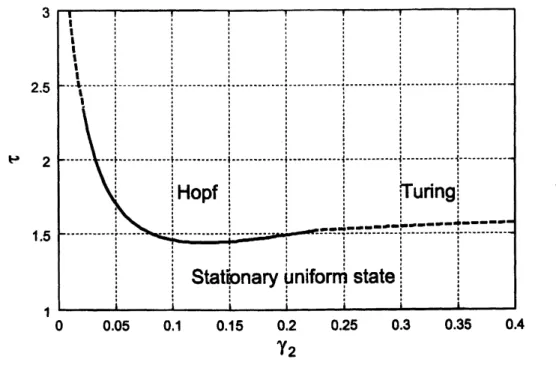
The linear stability diagramfor Eqs. (10) and (11) with Eqs. (13) and (14) in $\tau-\gamma_{2}$plane

is shown in Fig. 1for $D_{1}=1$, $\gamma_{1}=0.3$, and $\gamma_{3}=0.05$

.

Thesolid and dashed lnes in this

figure indicate the Hopfand Turing typeinstabilities, respectively. The stationary uniform

state is stable for the parameters below these lines.

III. NUMERICAL SIMULATIONS

In thissection,

we

shallshow,in

one

andtwodimensions, theresults obtainedbycomputer

simulations ofEqs. (10) and (11) with Eqs. (13) and (14) abovethe stability lines in Fig. 1.

First,

we

confirm numerically that apropagating solution exists in

one

dimension. The

space mesh and thetimeincrement have been set

as

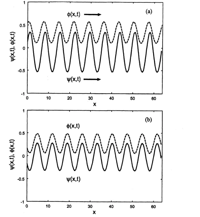
0.5 and0.001, respectively. Figure$2(\mathrm{a})$

shows suchasolution for$\tau=1.6$and $\gamma_{2}=0.15$, which isjust above the Hopf instabilityline

(thesolid line in Fig. 1). In Fig. 2(a) the profiles of$\psi(x, t)$ (solid line) and $\phi(x, t)$ (dashed

line)

are

plotted

as

functions of thespatialcoordinate$x$ at $t=5000$

.

Both profilesof$\psi(x,t)$

and $\phi(x,t)$ are moving to the right, in this case, at aconstant speed keeping their shapes

and the phase difference between them, whereas Fig. 2(b) depicts stationary patterns of$\psi$

and $\phi$without

a

phase difference for$\tau=1.6$and _{$\gamma_{2}=0.25$} above theTuring instability line.

A. Traveling lamellar pattern

Now

we

extend the simulations to two dimensions. The simulations have been carried

out

on

a128 $\mathrm{x}128$ square lattice with the mesh size $\Delta x=0.5$ using the finite difference

Euler scheme with afixed time step $At=10^{-3}$ _{for several values of parameters} $\tau$ and $\gamma_{2}$.

Other parameters are fixed at $D_{1}=1$, $\gamma_{1}=0.3$, and $\gamma_{3}=0.05$

.

As the initialconditions

we

start with homogeneous states with small randomperturbations which satisfy ($\psi\rangle=\psi_{0}$ and

$\langle\phi\rangle=\phi_{0}$ and used periodic boundary conditions, where theangle brackets

mean

the spatial

average.

As predicted bythelinearstabilityanalysis,

no

patternappears for theparameters below

the solid or dashed lines in Fig. 1. For the parameters above the dashed line at which the Turing-type instability occurs, stationary lamellar

or

hexagonal patternsappear depending

on the equilibrium values of$\psi_{0}$ and $\phi_{0}$

.

For theparameters abovethe Hopf-type instability

line(solidlinein Fig. 1), various travelingpatterns

are

observed. Henceforth,

we

concentrate

on

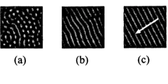
the parameter region near the Hopf instability line.

Figure 3displays threesnapshots of$\psi(\mathrm{r},t)$, indicated in gray scaleincreasing frombladc

to white, at $t=50(\mathrm{a})$, 500 (b), and 5000 (c) for _$\tau=1.6$ and $\gamma_{2}=0.2(\psi_{0}=$ -0.059,

$\phi 0=0.29)$. At the early stage irregular patterns with motions of distorted standing

waves

are

formed [Fig. $3(\mathrm{a})$]. After this transient regime, partially coherent lamellar structures

which aretravelingemerge [Fig. $3(\mathrm{b})$]. Thesystem eventuallyreaches the stateinwhich the

lamellar structure extended to the wholesystem is travelingat aconstant speed [Fig. $3(\mathrm{c})$].

The

arrows

in Fig. 3indicate the directions of propagation ofthe lamellar structures. The

behavior is similar to that reported by Hildebrandet al. [5] in thesurface chemical reaction

systems, although the evolution equations

are

quite different.

B. Traveling hexagonal pattern

One of the characteristic features ofthe present model system (10) and (11) with Eqs. (13) and (14) is that not onlylamellar pattern but also hexagonal structure

can

undergo a

coherent propagation by choosingthe values $\psi_{0}$ and $\phi_{0}$ appropriately.

Figure 4shows

one

example for $\psi_{0}=-0.20$, $\phi_{0}=0.40$ where three snapshots of$\psi(\mathrm{r},t)$

are

displayed in gray scale increasing from black towhite at $t=50(\mathrm{a})$, 500 (b), and

5000

(c) for $r$ $=1.6$ and $\gamma_{2}=0.1$

.

At the early stage, droplet-like domains irregularly

move

accompanied with breakups and coalescence of domains [Fig. $4(\mathrm{a})$, (b)] and finally form a

regular hexagonal pattern traveling in

one

direction at aconstant speed [Fig. $4(\mathrm{c})$]. The

propagatingdirection ofthe hexagons is indicated bywhite

arrows

in Fig. 4.

Another type of traveling hexagons appears

as

in Fig. 5where three snapshotsof$\psi(\mathrm{r},t)$,

at $t=50(\mathrm{a})$, 500 (b), and 5000 (c) are displayed for $\tau=2.0$ and $\gamma_{2}=0.06(\psi_{0}=-0.33$, $\phi_{0}=0.50)$. The transient behavior of this system is similar to that shown in Fig. 4.

However, the propagating direction (white arrows in this figure) at the asymptotic stateis

perpendicular to one ofthe primary wave vectors.

Thus, it is found that there are at least two different types of traveling hexagons.

Here-after,

we

call the

case

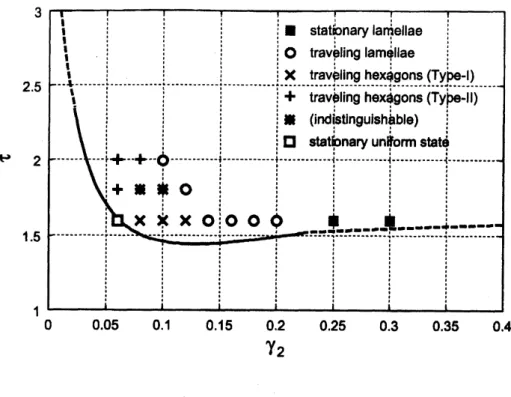
shown in Fig. 4the Type-I and in Fig. 5the Type-II, respectively.

The several ‘phases’ of nonequilibrium states have been obtained by carrying out the simulations for various parameters. Figure 6summarizes, in the parameter space $(\gamma_{2},\tau)$,

the various dynamic structures in two dimensions. Each symbol indicates, respectively,

stationary lamellar structure (closed squares), traveling lamellar structure (open circles),

traveling hexagonal structure of TypeI (crosses), travelng hexagonal structure of

Type-II (pluses), and uniform stable state (open square). For

some

parameters we could not

distinguish between Type-I and typeII hexagons within the present simulations. Such

parameters

are

plottedwithasterisksin Fig. 6. Inthis figure the Hopf andTuringinstability lines are also shown for convenience, which

are

the

same

asthose in Fig. 1.

It is noted here that the value of $\phi(\mathrm{r}, t)$, which is the

sum

ofthe local concentration of

$A$ and $B$ molecules, becomes negative in

some

parameter region. This shortcoming is due

to the simplification of the free energygiven by Eq. (9). However,

we

have carried out the simulations avoiding this parameter region and believe that the results obtained would not be altered even when

amore

refined free energy is employed.

The amplitude of the traveling

waves

is plotted in Fig. 7both for lamellar (open

cir-cles) and hexagonal (crosses) structures. It is evident that the bifurcation for lamellae is

supercritical whereas that for hexagons is subcritical.

$\mathrm{I}\mathrm{V}$

.

THEORETICAL ANALYSIS OF TRAVELING LAMELLAE

The computer simulations given in the previous section show that alamellar structure

exhibits aself-0rganized coherent propagation above the Hopf bifurcation threshold. It should be noted that astanding oscillation has

never

been observed in simulations. In order to understand this property,

we

derive the amplitude equation at post-threshold and examinethe stability of theoscillatory domains

A. Amplitude equation

We study the time-evolution equations (10)-(14) in

one

dimension

near

the Hopf

bifur-cation point at the critical wavenumber $q_{\mathrm{c}}$ in aweakly nonlinear regime. The amplitude

equation for Eqs. (10) and (11) near the Hopf instability line is derived by

means

of the

usualreductiveperturbationmethod $[21, 22]$ assumingthat the bifurcation_{is super-critical,}

which is indeed the

case as

has been shown in Fig.

7.

Near the bifurcation point, the most unstable mode $\mathrm{U}(x,t)$ is the relevant degrees of

freedom ofEqs. (10) and (11), that is, $\mathrm{u}\sim \mathrm{u}_{0}+\mathrm{U}$, where $\mathrm{u}\equiv(\psi, \phi)^{T}$ and $\mathrm{u}_{0}\equiv(\psi_{0}, \phi_{0})^{T}$

.

In terms of the eigen functions $\mathrm{U}_{L}$ and $\mathrm{U}_{R}$ defined below, the unstable mode $\mathrm{U}(\mathrm{x}$, is

expressed

as

$\mathrm{U}(x,t)=W_{L}(x,t)\mathrm{U}_{L}+WR(x,t)$ $+\mathrm{c}.\mathrm{c}$

.

(21) where $\mathrm{c}.\mathrm{c}$

.

denotes the complex conjugate and $Wi,(x,t)$ and $W_{R}(x,t)$

are

the complex

am-plitudesof theplanewavesolution propagating to theleft andright, respectively. The

wave

number$q_{\mathrm{c}}$and the frequency$\omega_{\mathrm{c}}$ of theplane

wave

are

determinedbytheeigenvalue problem:

$(\partial_{t}-\mathcal{L}_{q_{\mathrm{c}}})\mathrm{U}_{L}=0$, (22)

where $\partial_{t}$ denotes the partial differential operator with respect to

$t(\mathrm{U}_{R}$ also satisfies the

same

equation). For the present problem we choose

$\mathrm{U}_{L}=(\begin{array}{l}1\alpha\end{array})$ $\mathrm{e}^{iq_{e}x+\dot{u}d_{\mathrm{C}}t}$

$\mathrm{U}_{R}=(\begin{array}{l}1\alpha\end{array})$ $\mathrm{e}^{-\dot{\eta}_{e}x+\dot{*}\omega_{\mathrm{C}}t}$

(23)

with $\alpha\equiv(a_{22}+i\omega_{c})/a_{12}$ and $\omega_{\mathrm{c}}(>0)$ is given by

$\omega_{\mathrm{c}}^{2}=\det \mathcal{L}_{q_{\mathrm{C}}}=-a_{22}^{2}-a_{12}a_{21}$ (21)

By the standard procedure of the perturbation $[21, 22]$, the final amplitude equations for

$W_{L}$ and $W_{R}$

are

given, respectively, by

$\partial_{t}W_{L}=\mu W_{L}+b\partial_{x}^{2}W_{L}-g|W_{L}|^{2}W_{L}-h|W_{R}|^{2}W_{L}$, (23)

$\partial_{t}W_{R}=\mu W_{R}+b\partial_{x}^{2}W_{R}-g|W_{R}|^{2}W_{R}-h|W_{L}|^{2}W_{R}$, (26)

where all the coefficients

are

complexand

are

given by

$\mu\equiv\frac{\tilde{\tau}}{2}q_{\mathrm{c}}^{2}(1+\frac{ia_{22}}{\omega_{\mathrm{c}}})$, (27)

$b \equiv 2D_{1}q_{c}^{2}(1+\frac{ia_{22}}{\omega_{\mathrm{c}}})$, $g \equiv\frac{3}{2}q_{c}^{2}(1+\frac{ia_{22}}{\omega_{c}})[1+24\psi_{0}^{2}q_{\mathrm{c}}^{2}\frac{a_{22}-2i\omega_{c}}{9(a_{11}+a_{22})(a_{22}-2i\omega_{\mathrm{c}})-3\omega_{c}^{2}}]$, $h \equiv 3q_{\mathrm{c}}^{2}(1+\frac{ia_{22}}{\omega_{\mathrm{c}}})[1+24\psi_{0}^{2}q_{\mathrm{c}}^{2}\frac{a_{22}}{9(a_{11}+a_{22})a_{22}+\omega_{\mathrm{c}}^{2}}]$ , (28) (29) (30)

and $\tilde{\tau}\equiv\tau-\tau_{\mathrm{c}}$with acritical value $\tau_{\mathrm{c}}$ of$\tau$ at which the bifurcation

occurs.

The constant $g$

should not be confusedwiththefunction inEq. (14). Thistypeofamplitude equations

was

also obtained in Refs. $[23, 24]$

.

Notethat Eqs. (25) and (26) do not have terms proportional

to$\partial_{x}W_{L}$ or $\partial_{x}W_{R}$. Thisreflects the fact thatin

our

model thegroupvelocityis alwayszero, that is, $d\omega(q_{c})/dq=0$, where $\omega(q)\equiv\sqrt{\det \mathcal{L}_{q}}$

near

the bifurcation point. This

comes

from

the particular choice of$D_{2}=0$ in Eq. (3).

B. Stability of traveling wave

Here

we

examine stability of the traveling

wave

solution of Eqs. (25) and (26). These

equationshave aset of solutions $W_{L}^{(0)}$ and $W_{R}^{(0)}$

as

$W_{L}^{(0)}=0$, $W_{R}^{(0)}=N_{0}\mathrm{e}^{-\dot{|}qx+\mathrm{f}\mathrm{f}1_{0}(q)t}$, (31)

where the realconstants $\Omega_{0}$ and $N_{0}$

are

given by

$N_{0}^{2}= \frac{1}{g_{1}}(\mu_{1}-b_{1}q^{2})$, (32) $\Omega_{0}=\mu_{2}-b_{2}q^{2}-\frac{g_{2}}{g_{1}}(\mu_{1}-b_{1}q^{2})$, (33)

and $\mu=\mu_{1}+\mathrm{i}12$, $b=b_{1}+ib_{2}$ with real numbers $\mu_{1}$, $\mu_{2}$, $b_{1}$ and $b_{2}$

.

Asimilar notation has

also been utilized for$g$ and $h$

.

In orderto studythe stability ofthe solution (31), let us introduce deviations

_4and

$\eta$ as

$W_{L}=W_{L}^{(0)}+\xi$, (34) $W_{R}=W_{R}^{(0)}+\eta$

.

(35)

Substituting Eqs. (34) and (35) into Eqs. (25) and (26) yields up to the first order ofthe

deviations

$\partial_{t}\xi=\mu\xi+b\partial_{x}^{2}\xi-hN_{0}^{2}\xi$, (36) $\partial_{t}\eta=\mu\eta+b\partial_{x}^{2}\eta-(W_{R}^{(0)})^{2}\overline{\eta}-2gN_{0}^{2}\eta$, (37)

where $\overline{\eta}$ is the complex conjugate to

$\eta$. Setting$\xi\propto\exp(iqx+\lambda t)$, we obtain

A $=\mu-bq^{2}-hN_{0}^{2}$

.

(38)

The growth rate of the deviation

_4is

given by

$\mathrm{R}\epsilon$ A

$=( \mu_{1}-b_{1}q^{2})(1-\frac{h_{1}}{g_{1}})$, (39)

where

we

have used Eq. (32). Since $(\mu_{1}-b_{1}q^{2})/g_{1}=N_{0}^{2}>0$,weneed thestabilitycondition

for the traveling

wave

$[23, 24]$

$h_{1}>g_{1}$

.

(40)

Next,

we

investigate stability of the standing

wave

solution given by

$W_{L}^{(0)}=N_{0}\mathrm{e}^{\dot{|}}qx+\dot{l}\Omega_{0}l$, $W_{R}^{(0)}=N_{0}\mathrm{e}^{-\dot{\eta}x+\cdot\Omega_{0}t}.$, (41)

where $\Omega_{0}$ and $N_{0}$ satisfythe following relation,

$i\Omega_{0}=\mu-bq^{2}-gN_{0}^{2}-hN_{0}^{2}$

.

(42)

We introduce the small deviations of the amplitudes $\xi(x, t)$, $\eta(x, t)$ and the phases $\varphi(x, t)$,

$\theta(x,t)$

as

$W_{L}=N_{0}(1+\xi)\mathrm{e}^{\dot{\eta}x+\cdot\Omega_{\mathrm{O}^{\mathrm{Z}+\dot{1}}}\varphi}.$, (43)

$W_{R}=N_{0}(1+\eta)\mathrm{e}^{-:}qx+|.\Omega_{0}t+\cdot.\theta$, (44)

From Eqs. (25), (26), (43) and (44)

we

obtain the time evolution equationsforthedeviations.

Thedeviations of amplitudes obey up to the first order

$\partial_{t}\xi=-2g_{1}N_{0}^{2}\xi-2h_{1}N_{0}^{2}\eta+b_{1}\partial_{x}^{2}\xi-2qb_{2}\partial_{x}\xi-2qb_{1}\partial_{x}\varphi-b_{2}\partial_{x}^{2}\varphi$ , (43) $\partial_{t}\eta=-2g_{1}N_{0}^{2}\eta-2h_{1}N_{0}^{2}\xi+b_{1}\partial_{x}^{2}\eta+2qb_{2}\partial_{x}\eta+2qb_{1}\partial_{x}\theta-b_{2}\partial_{x}^{2}\theta$, (46)

where we have used Eq. (42). In the long-wave-length limit, we may retain only the first

two terms of Eqs. (45) and (46). In this case, the eigenvalues of the time evolution matrix

are

A$=-2N_{0}^{2}(g_{1}\pm h_{1})$

.

(47)

Since

$g_{1}$ is positive when the bifurcation is super-critical,

we

have the stability conditionof the standing

wave

$[23, 24]$

$-g_{1}<h_{1}<g_{1}$. (48)

According to the numericalcalculations based

on

Eqs. (29) and (30), we havenot found the

parameters for which the standing wave is stable

as

long as $g_{1}>0$. This agrees with the

fact that we have never found the standing wave in the simulations ofEqs. (10)-(14).

C. Phase dynamics for traveling wave

Now we discuss phase dynamics for the traveling

wave

solution. We write asolution of Eqs. (25) and (26) withthe deviations $\xi(x,t)$ and $\varphi(x,t)$

as

$W_{L}=0$, $W_{R}=N_{0}(1+\xi)\mathrm{e}^{-\dot{\eta}x+\dot{\iota}\Omega_{0}t+\dot{|}\varphi}$

.

(49) Thezeroth-0rder solution has been obtained in Eqs. (31). The first order equations

are

given by

$\partial_{t}\xi=-2g_{1}N_{0}^{2}\xi+b_{1}\partial_{x}^{2}\xi+2qb_{2}\partial_{x}\xi+2qb_{1}\partial_{x}\varphi-b_{2}\partial_{x}^{2}\varphi$, (50) $\partial_{t}\varphi=-2qb_{1}\partial_{x}\varphi+b_{1}\partial_{x}^{2}\varphi+b_{2}\partial_{x}^{2}\xi+qb_{2}\partial_{x}\varphi-2g_{2}N_{0}^{2}\xi$. (51)

Sincetheamplitude deviation decays rapidly compared withthephasedeviationin the long

wave

engthmodulation,

we

may eliminate 4adiabaticallyby putting$\partial_{t}\xi=0$in Eq. (50)

so

that wehave

$\xi=\frac{1}{2g_{1}N_{0}^{2}}(2qb_{1}\partial\varphi-b_{2}\partial_{x}^{2}\varphi+2qb_{2}\partial_{x}\xi+b_{1}\partial_{x}^{2}\xi)$

.

(52) Applying Eq. (52)iteratively,

we

obtainthe followingexpression of$\xi$

as

gradientexpansion of$\varphi[23,24]$,

$\xi=\frac{qb_{1}}{g_{1}N_{0}^{2}}\partial_{x}\varphi+\frac{b_{2}}{2g_{1}N_{0}^{2}}(-1+\frac{2q^{2}b_{1}}{g_{1}N_{0}^{2}})\partial_{x}^{2}\varphi+\cdots$

.

(53)

Substituting Eq. (53) into Eq. (51) we obtain up tothe second-0rder derivatives of $\phi$

$\partial_{t}\varphi=C\partial_{x}\varphi+D\partial_{x}^{2}\varphi$, (54) where

$C \equiv 2q(b_{2}-\frac{g_{2}}{g_{1}}b_{1})$, (55)

$D \equiv(b_{1}+\frac{g_{2}}{g_{1}}b_{2})(1-\frac{2q^{2}b_{1}}{g_{1}N_{0}^{2}})$

.

(56)

Here

we

consider the

case

that the factor $b_{1}+g_{2}b_{2}/g_{1}$ in Eq. (56) is positive

so

that the

traveling

wave

solutionisstable for $|q|arrow \mathrm{O}$

.

In thiscase, the

coefficient

$D$ becomesnegativ

for large value of $|q|$, which

causes an

Ekhaus-type instability.

Since

_{$1-2q^{2}b_{1}/(g_{1}N_{0}^{2})=$} $(\mu_{1}-3q^{2}b_{1})/(g_{1}N_{0}^{2})$, this instability

occurs

when

$q^{2}> \frac{\mu_{1}}{3b_{1}}$. (57)

Note that the condition $q^{2}<\mu_{1}/b_{1}$ isrequired for the traveling

wave

solution to exist.

We

can

obtainamplitude equations_{for the traveling lamellar structures which}

_are

_similar

totheequationfor theonedimensionalcase. The complex amplitudes $W_{L}(\mathrm{r}, t)$ and $W_{R}(\mathrm{r},t)$

of

waves

propagating to the left and right in $x$-direction obey the following equations,

cor-responding to Eqs. (25) and (26),

$\partial_{t}W_{L}=\mu W_{L}+b(\partial_{x}-\frac{i}{2q_{\mathrm{c}}}\partial_{y}^{2})^{2}W_{L}-g|W_{L}|^{2}W_{L}-h|W_{R}|^{2}W_{L}$ , (58)

$\partial_{t}W_{R}=\mu W_{R}+b(\partial_{x}-\frac{i}{2q_{\mathrm{c}}}\partial_{y}^{2})^{2}W_{R}-g|W_{R}|^{2}W_{R}-h|W_{L}|^{2}W_{R}$, (59)

wherethe coeflBcients $\mu$, $b$, $g$, and $h$

are

defined in Eqs. (27)-(30).

We

can

also develop the phase dynamics in two dimensions from the above amplitude

equation. Wewrite atravelingwavesolution ofEqs. (58) and (59) propagating to x-direction

as

$W_{L}=0$, $W_{R}=N_{0}[1+\xi(\mathrm{r},t)]\mathrm{e}^{-|qx+:\Omega_{0}t+|\varphi(\mathrm{r},t)}..$, (60)

where $\xi(\mathrm{r},t)$ and $\varphi(\mathrm{r}, t)$

are

the small

deviations

associated with theamplitude and phase,

respectively. Repeating the same procedure _shown above, we obtain the phase equation

correspondingto Eq. (54)

as

$\partial_{t}\varphi=C\partial_{x}\varphi+D\partial_{x}^{2}\varphi-\frac{q}{q_{C}}(b_{1}+\frac{g_{2}}{g_{1}}b_{2})\partial_{y}^{2}\varphi$, (61) where $C$ and $D$

are

given by Eqs. (55) and (56), respectively. Equation (61) implies that

when $q>0$ the phase deviation in $y$-direction is destabilized. This corresponds to the

zig-zag-type instability.

In the numericalsimulations shownin Sec. IIIwehave

never

found boththe Ekhaus- and

the zig-zag-type

instabilities.

We should say that the traveling

wave

solution is quitestable

in

our

modelsystem.

V. THEORETICAL ANALYSIS OF TRAVELING HEXAGONS

In twodimensional systems, notonly alamelar structure but also ahexagonalstructure

are

allowed to exist

as

aspatially periodicstructure. As

was

shown in the previous section

the hexagonal structure also undergoes acoherent propagation above the Hopf instability line.

We do not carry out asystematic derivation ofthe amplitude equations for the traveling

hexagons mainly because the bifurcation is subcritical and hence evaluation of each

coeffi-cient of the amplitude equation is

more

involved. Here we employ asimple modeexpansion

focusing

on

the two types ofthe traveling pattern obtained inthe simulations.

We seek asolution of Eqs. (10) and (11) in the following form, $\psi(\mathrm{r}, t)=\hat{\psi}(\mathrm{r}-\mathrm{V}t)$, $\phi(\mathrm{r},t)=\hat{\phi}(\mathrm{r}-\mathrm{V}t)$, with atraveling velocity V. Here we make theapproximation that the functions $\hat{\psi}(\mathrm{r})$ and $\hat{\phi}(\mathrm{r})$

are

represented in terms of the lowest Fourier modes as

$\hat{\psi}(\mathrm{r})=\sum_{k=-3}^{3}\hat{\psi}_{\mathrm{q}k}e^{\mathrm{q}_{k}\cdot \mathrm{r}}.\cdot$, $\hat{\phi}(\mathrm{r})=\sum_{k=-3}^{3}\hat{\phi}_{\mathrm{q}k}e^{\dot{l}\mathrm{q}_{k}\cdot \mathrm{r}}$, (62)

where $\mathrm{q}_{k}\equiv(q_{\mathrm{c}}\cos\frac{2\pi}{3}k, q_{\mathrm{c}}\sin\frac{2\pi}{3}k)(k=\pm 1, \pm 2, \pm 3)$and $\mathrm{q}_{0}\equiv 0$. Note that $\hat{\psi}_{\mathrm{q}0}=\psi_{0}$, and

$\hat{\phi}_{\mathrm{q}0}=\phi_{0}$

.

We have verified numerically that $\mathrm{t}\mathrm{h}\dot{\mathrm{e}}$ actual spatial profile is not substantially

deviated from Eq. (62)

near

the Hopfbifurcation line although it is subcritical.

PromEqs. (10), (11) and (62),

we

obtain aset ofequationfor$\hat{\psi}_{\mathrm{q}k},\hat{\phi}_{\mathrm{q}k}$ and V. Eliminating

$\hat{\phi}_{\mathrm{q}k}$ and introducing areal amplitude _{$A_{k}$} and aphase $\theta_{k}$

as

$\hat{\psi}_{\mathrm{q}\mathrm{k}}=A_{k}\exp(i\theta_{k})$,

we

finally obtain

$\Omega(\omega_{k})A_{k}=\mu A_{k}-3q_{\mathrm{c}}^{2}[2\psi_{0}A_{l}A_{m}e^{-\dot{l}}\varphi+A_{k}^{3}+2(A_{l}^{2}+A_{m}^{2})A_{k}]$ (63)

for $k=1,2,3(l,m=k+1, k+2(\mathrm{m}\mathrm{o}\mathrm{d} 3))$ with

$\Omega(\omega)\equiv\frac{\omega^{2}-\omega_{c}^{2}}{\omega^{2}+a_{22}^{2}}(a_{22}-i\omega)$, (64)

where$\varphi\equiv\theta_{1}+\theta_{2}+\theta_{3}$, $\mu\equiv-q_{\mathrm{c}}^{2}(Dq_{\mathrm{c}}^{2}-\tilde{\tau})-(\gamma_{1}+\gamma_{2}+\gamma_{3})$,$\omega_{k}\equiv \mathrm{q}_{k}\cdot \mathrm{V}$, and$\omega_{\mathrm{c}}\equiv{\rm Im}\lambda(q_{c})$ isthe

criticalfrequency at the Hopfbifurcation point. Notethat two ofthe three phase variables

$\theta_{k}$

are

arbitrary and only the

sum

$\varphi$is determined bythe aboveequations. Therefore, Eqs. (63) and (64) under the condition$\omega_{1}+\omega_{2}+\omega_{3}=0$ determine $A_{\mathrm{k}}$,

$\varphi$, and V. When $A_{k}\neq 0$, the imaginary part ofEq. (63) gives

$- \omega_{k}\frac{\omega_{k}^{2}-\omega_{\mathrm{c}}^{2}}{\omega_{k}^{2}+a_{22}}=6q_{c}^{2}\psi_{0}\frac{A_{l}A_{m}}{A_{k}}\sin\varphi$

.

(65)

In the special case that $\sin\varphi=0$, Eq. (65) has solutions $\omega_{k}=0$ and $\pm\omega_{\mathrm{c}}$

.

If

we

choose $\omega_{1}=0$, $\omega_{2}=\omega_{\mathrm{c}}$, and $\omega_{3}=-\omega_{\mathrm{c}}$, then the traveling velocity

$\mathrm{V}$ is perpendicular to

$\mathrm{q}_{1}$ [see

Fig. $8(\mathrm{a})]$

.

This is the Type-I solution. Ontheother hand,the Type-II solution ofEqs. (63)

is represented

as

$\omega_{1}=-2\omega_{2}$ and $\omega_{2}=\omega_{3}$ which satisfiesthe condition $\omega_{1}+\omega_{2}+\omega_{\theta}=0$

.

In

this case, $\mathrm{V}$ is indeed parallel to

$\mathrm{q}_{1}$

as

shown in Fig. $8(\mathrm{b})$

.

VI. CONCLUDING REMARKS

In this paper,

we

haveconstructed the model equation for phase separationofchemically

reactive ternary mixtures. In this model the thermodynamic destabilization induces the

Turing- or Hopf-type instability at afinite

wave

number depending

on

the parameters in

the reaction terms. The phase diagram for the nonequilibrium states has been obtained numerically. Traveling

waves

appear

as

aHopfbifurcation at afinite wavenumber. In two

dimensional simulations

we

have obtained the traveling lamellar structure and two types

(Type-I and types I) of traveling hexagonal structures. The mathematical structure of

these two types of traveling hexagons has been investigated by the amplitude equations

derivedbythe singlemodeapproximation. Whatwehave showninthis paper isthat phase

transitions in anon-equilibrium condition produce arich variety of self-0rganized domain

dynamics which never

occur

in thermal equilibrium where the ordered state is motionless

and is simply uniform or at most modulated in space.

We have derivedthe amplitude equationsforthesupercritical Hopfbifurcationat afinite

wavenumber from the model equations and investigated the stability of the traveling

wave

and the standing oscillation in$\mathrm{o}\mathrm{n}\triangleright$ imensional systems. The traveling

wave

is found to be

stable in

some

parameter regions.

However

we

have

never

found, at least numerically, any

region in which the standingoscillation is stable.

There is asimple explanation

as

to why one needs threecomponents ofchemical species

forcoherently propagatingdomains. Suppose that thespeciesarearrayed inonedimensional

space

as

$A$, $B$, $C$, $A$

.

After

one

cycle ofchemical reaction, this order becomes $B$, $C$, $A$, $B$

.

This

means

that domains

are

moving to the left. It is clear from this argument that the

relative phase difference of the chemical reaction determines the propagating direction and

that astanding oscillation isquite unlikely in thepresent system.

Thermal fluctuations have been believed to be unimportant for pattern formation far

from equilibrium

as

long

as

macroscopic patterns such

as

Rayleigh-B6nard convection and

Belousov-Zhabotinski

reaction

are

concerned. (See, however, recent experiments [25] for

electroconvection of liquid crystals.) On the contrary, when the domain structure is of

microscopic scale

as

in the present model system, thermal fluctuations cannot be ignored

near

the bifurcationpointsout of equilibrium and might alter qualitatively the properties of

thetransition. Concentration fluctuations around thedeterministic motion may also exhibi

somecharacteristic features inherent to non-equilibriumsystems. Wehopeto return tothese fundamental problems elsewhere in the future.

Acknowledgments

We would like to thank Professor A. S. Mikhailov for valuable discussions. This work

was

supported by the Grant-in-Aid for Scientific Research from the Ministry ofEducation,

Science, Sports and Culture of Japan.

[1] M. C. Cross and P. C. Hohenberg, Rev. Mod. Phys. 65, 851 (1993).

[2] A. Joets andR. Ribotta, Phys. Rev. Lett. 60, 2164 (1988).

[3] R. Imbihl and G. Ertl, Chem. Rev. 95, 697 (1995).

[4] A. vonOertzen, H. H. Rotermund, A. S. Mikhailov and G. Ertl, J. Phys. Chem. $\mathrm{B}104$,3155

(2000).

[5] M. Hildebrand, A. S. Mikhailov, and G. Ertl, Phys. Rev. Lett. 81, 2602 (1998).

[6] A. S. Mikhailov, M. Hildebrand, and G. Ertl, in Coherent Structures in Classical Systems,

edited by M. Rubi et al. (Springer, NewYork, 2001) and references cited therein.

[7] Y. Tabe and H. Yokoyama, Langmuir 11, 4609 (1995).

[8] R. Reigada, F. Sagues, and A. S. Mikhailov, unpublished.

[9] S. C. Glotzer, E. A. Di Marzio, and M. Muthukmar, Phys. Rev. Lett. 74, 2034 (1995).

[10] J. Verdasca, P. Borckmans, andG. Dewel, Phys. Rev. $\mathrm{E}52$, R4616 (1995).

[11] M. Motoyama andT. Ohta, J. Phys. Soc. Jpn., 66, 2715 (1997).

[12] Q. Tran-Cong and A. Harada, Phys. Rev. Lett. 76, 1162 (1996).

[13] T. Ohta and K. Kawasaki, Macromolecules 19, 2621 (1986).

[14] M. BahianaandY. Oono, Phys. Rev. A41, 6763 (1990).

[15] J.D. Gunton,M. San Miguel, and P.S. Sahni, in Phase Transitionsand CriticalPhenomena,

edited by C. Domb and J. L. Lebowitz (Academic Press, NewYork, 1983) Vol. 8.

[16] A. J. Bray, Adv. Phys. 43, 357 (1994).

[17] I. Daumont, K. Kassner, C. Misbah, and A. Valance, Phys. Rev. $\mathrm{E}55$,6902 (1997).

[18] C. B. Price, Phys. Rev. $\mathrm{E}55$,6698 (1997).

[19] T. Okuzono andT. Ohta, Phys. Rev. $\mathrm{E}64$,045201 (2001).

[20] E. M. Nicola, M. Or-Guil, W. Wolf, and M. Bi, Phys. Rev. $\mathrm{E}65$,055101 (2002).

[21] Y. Kuramoto, Chemical Oscillations, Waves and Turbulence (Springer-Verlag, Berlin, 1984).

[22] D. Walgraef, SpatiO-Temporal PatternFormation (Springer-Verlag,NewYork, 1997).

[23] P. Coullet, S. Fauve, and E. Tirapegui, J. Physique Lett. 46, L-787 (1985).

[24] T. Ohta and K. Kawasaki, Physica $27\mathrm{D}$, 21 (1987).

[25] M. A. Schererand G. Ahlers, Phys. Rev. $\mathrm{E}65$,051101 (2002).

Y2

FIG. 1: Linear stabilitydiagram for Eqs. (10) and (11) with Eqs. (13) and (14) in $\mathcal{T}\neg 2$ plane for

$D_{1}=1$, $\gamma_{1}=0.3$, and $\gamma_{3}=0.05$. Thesolid anddashed lines in this figure indicate the Hopfand

Turing type instabilities, respectively

–

$\hat{\mathrm{x}}$ $\check{\mathrm{e}-}$ $\overline{\mathrm{x}^{-}}-$ $\vee\geq$ $\mathrm{x}$ $\hat{\overline{\vee\Leftrightarrow\tilde{\mathrm{x}}}}$ $\overline{\mathrm{x}^{-}}-$ $\vee\geq$ $\mathrm{x}$

FIG. 2: Spatial profilesof

₉

$(x,t)$(solid lines) and$\phi(x,t)$ (dashedlines)obtained byone- imensional

simulations for (a) $\tau=1.6$, $\gamma_{2}=0.15$ (just above the Hopf instability line) and (b) _$\tau=1.6$,

$\gamma_{2}=0.25$ (just above the Turing instability line) at _$t=5000$. Both profilesof$\mathrm{r}\mathrm{p}(\mathrm{x},\mathrm{t})$ and$\mathrm{r}\mathrm{p}(\mathrm{x},\mathrm{t})$

are propagating to $x$-direction indicated by the arrow with the same velocity in the case of (a),

whereas theyare stationaryin the caseof (b)

(a) (b) (c)

FIG. 3: Snapshots of $\psi(\mathrm{r}, t)$, indicated in gray scale increasing from black to white, at $t=50$

(a), 500 (b), and 5000 (c) for $\tau$ $=1.6$ and $\gamma_{2}=0,2$

.

The white arrow indicates the direction of

propagation of the lamellar structure.

(a) (b) (c)

FIG. 4: Snapshots of$\psi(\mathrm{r}, t)$ indicated ingrayscale increasing fromblackto whiteat$t=50(\mathrm{a})$,500

(b), and5000 (c) for $\tau=1.6$ and$\gamma_{2}=0.1$. The white arrow indicatesthe direction of propagation

of the hexagonal structure (Type$\mathrm{I}$).

(a) (b) (c)

FIG. 5: Snapshots of$\psi(\mathrm{r}, t)$ indicatedingrayscale increasing from black to white at$t=50(\mathrm{a})$, 500

(b), and5000 (c)for $\tau=2.0$and$\gamma_{2}=0.06$

.

The white

arrow

indicatesthedirection of propagation

of the hexagonal structure (Type- $\mathrm{I}$).

$\mathrm{P}$

$\gamma_{2}$

FIG. 6: Parameterdependence ofthenonequilibriumstatesin$(\gamma_{2},\tau)$space. Each symbolindicates,

respectively, stationary lamellar structure (closed squares), traveling lamellar structure (open

cir-cles), traveling hexagonal structure ofType-I (crosses), traveling hexagonal structure of Type-II

(pluses), and stationaryuniform state (open square). Theasterisks meanthe states thatwecould

not distinguish between Type-I and Type-II hexagons within the present simulations. The Hopf

andTuringinstability lines arealso shown for convenience, which arethe same asthose inFig. 1.

$\tau$

FIG. 7: Amplitudesof$\psi$ in the travelng state forthelamellar (open circles) $[\gamma_{1}=0.3,$ $\gamma_{2}=0.2$,

and$\gamma_{3}=0.05$] and hexagonal (crosses) [$\gamma_{1}=0.3,$ $\gamma_{2}=0.1$, and $\gamma_{3}=0.05$] structures asfunctions

of the control parameter $\tau$

.

$\ovalbox{\tt\small REJECT}$ $\mathrm{q}_{1}$ $\ovalbox{\tt\small REJECT}$ $\ovalbox{\tt\small REJECT}$ $\mathrm{q}_{1}$ $\ovalbox{\tt\small REJECT}$ (a) (b)

FIG. 8: Schematicpicture of the directions oftraveling velocity$\mathrm{V}$andwavevector

$\mathrm{q}_{1}$ fortraveling

hexagonaldomains ofType-I (a) andTypeII (b). Thick and thin

arrows

indicate the directionof

$\mathrm{V}$and

$\mathrm{q}_{1}$, respectively, andthe hatched regions represent

$\psi$-rich domains