ON THE RANGE OF THE FIRST TWO DIRICHLET
EIGENVALUES OF THE LAPLACIAN WITH VOLUME AND
PERIMETER CONSTRAINTS
PEDRO R. S. ANTUNES AND ANTOINE HENROT
ABSTRACT. In this paper we study the set of points, in the plane, defined
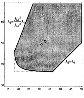
by $\mathcal{E}^{A}:=\{(x, y)=(\lambda_{1}(\Omega), \lambda_{2}(\Omega)), |\Omega|=1\}$ on the one hande and $\mathcal{E}^{P};=$
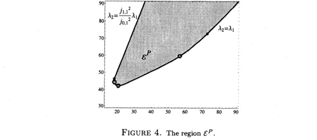
$\{(x, y)=(\lambda_{1}(\Omega), \lambda_{2}(\Omega)), P(\Omega)=2\sqrt{\pi}\}$,ontheotherhandwhere$(\lambda_{1}(\Omega), \lambda_{2}(\Omega))$
arethe two first eigenvalues of theDirichlet-Laplacian. We givesome
qualita-tive propertiesof thesesets and showsomepicturesobtained through
numer-ical computations.
1. INTRODUCTION
Let $\Omega\subset \mathbb{R}^{2}$ be a bounded open set, $|\Omega|$ its area and $P(\Omega)$ its perimeter. Let us
consider the Dirichlet eigenvalue problem,
(1) $\{\begin{array}{ll}-\Delta u=\lambda u in \Omega u=0 on \partial\Omega,\end{array}$
definedonthe Sobolevspace $H_{0}^{1}(\Omega)$
.
We will denote the eigenvalues by$0<\lambda_{1}(\Omega)\leq$$\lambda_{2}(\Omega)\leq\ldots$ (counted with their multiplicities) and the corresponding orthonormal
real eigenfunctions by $u_{i},$ $i=1,2,$$\ldots.$
A natural question in spectral geometry is the following:
let$0<a\leq b$ be two given realnumbers, does there exist a domain$\Omega$
of
area
1 whichhas $a$ and $b$ as their two
first
eigenvalues? In acoustic, the question corresponds to:is there exist a drum of given
area
(say 1) whose two first fundamental frequenciesare $a$ and $b?$
.
In [WK] and [BBF], itwas
studied the region$\mathcal{E}^{A}=\{(x, y)\in \mathbb{R}^{2}:(x, y)=(\lambda_{1}(\Omega), \lambda_{2}(\Omega)), \Omega\subset \mathbb{R}^{2}, |\Omega|=1\},$
which is therange of the first two Dirichlet eigenvaluesofplanar setswithunit
area.
We also refer to [LY] for a similar study for the three first eigenvalues. Obviously,
the completeknowledge of theset $\mathcal{E}^{A}$ allows to answer theprevious questions. The
same question can be raised by replacing the area by the perimeter. It leads to
study the set
$\mathcal{E}^{P}=\{(x, y)\in \mathbb{R}^{2}:(x, y)=(\lambda_{1}(\Omega), \lambda_{2}(\Omega)), \Omega\subset \mathbb{R}^{2}, P(\Omega)=2\sqrt{\pi}\},$
Date: March 14, 2013.
1991 Mathematics Subject Cassification. Primary $35P15$; Secondary$58G25.$
Key words and phrases. Dirichlet Laplacian, eigenvalues, shape optimization.
The work of P.$A$. is partially supported by FCT, Portugal, through the
schol-arship SFRH/BPD/47595/2008, and the scientific projects PTDC/MAT/101007/2008,
PTDC/MAT/105475/2008 and PEst-$OE/MAT/UI0208/2011$
.
The work of Antoine Henrot ispart of the project ANR-12-$BS$01-0007-01-OPTIFORM Optimisation deformesfinanced by the
These two questions will be discussed in this paper.
The plan of this paper is the following. In the next section we study the set
$\mathcal{E}^{A}$ and
we mainly recall results already contained in [WK], [BBF] and [BNP] with
some
proofs. Then insection 3, we study the set$\mathcal{E}^{P}$ and givesomeof its properties,
2. THE RANGE OF $\{\lambda_{1},$$\lambda_{2}\}$ WITH AN AREA CONSTRAINT
We recall that
we
want to study the set$\mathcal{E}^{A}=\{(x, y)\in \mathbb{R}^{2}:(x, y)=(\lambda_{1}(\Omega), \lambda_{2}(\Omega)), \Omega\subset \mathbb{R}^{2}, |\Omega|=1\},$
Let us begin with
some
elementary facts. Obviously $\mathcal{E}^{A}$ liesin the first quadrant and within the sector $0<x\leq y$, because we defined the eigenvalues to be ordered.
The behavior of eigenvalues with respect to homothety $(\lambda_{k}(t\Omega)=\lambda_{k}(\Omega)/t^{2})$ has
two consequences. First we can also write
(2) $\mathcal{E}^{A}=\{(x, y)\in \mathbb{R}^{2}:(x, y)=(\lambda_{1}(\Omega), \lambda_{2}(\Omega)), \Omega\subset \mathbb{R}^{2}, |\Omega|\leq 1\}$
(3) $\{(x, y)\in \mathbb{R}^{2}:(x, y)=(|\Omega|\lambda_{1}(\Omega), |\Omega|\lambda_{2}(\Omega)), \Omega\subset \mathbb{R}^{2}\}.$
Moreoverthe region $\mathcal{E}^{A}$
is conical with respect to the origin in the sense,
$(x, y)\in \mathcal{E}^{A}\Rightarrow(\alpha x, \alpha y)\in \mathcal{E}^{A}, \forall\alpha\geq 1.$
Indeed, we can consider a homothety of ratio $1/\sqrt{\alpha}$ of the original domain and
complete with a collection of small balls to reach volume 1 without changing the
two first eigenvalues. This proves also the first equality in (2).
Now, we can get more precise information about $\mathcal{E}^{A}$ thanks to
some important
results on the low eigenvalues of the Laplacian. This region can be reduced using
thefamous Faber-Krahn inequality proved in [Fl] and [K], $(see [H,$ Theorem$3.2.1])$
which states that the ball minimizes $\lambda_{1}$ among all planar domains with the
same area. We can write this result as
$|\Omega|\lambda_{1}(\Omega)\geq\lambda_{1}(\mathcal{B})=\pi j_{0,1}^{2}\approx 18.16842,$
where $j_{n,k}$ denotes the k-th positive zero of the Bessel function $J_{n}$ and $\mathcal{B}$ denotes
the ball ofunit
area.
Equality holds if and only if$\Omega$ is a ball (up to.a set ofzerocapacity). For the second eigenvalue, we know that the minimum is attained by
two balls of equal
area.
This result is due to Krahn and has been rediscovered bySzeg\"o, and
some
other authors, see [$H$, Theorem 4.1.1] for more details. It can bewritten as
$|\Omega|\lambda_{2}(\Omega)\geq 2\lambda_{1}(\mathcal{B})=2\pi j_{0,1}^{2}\approx 36.33684.$
The quotient $\lambda_{2}/\lambda_{1}$ is maximized at the ball $(cf. [AB1] or [H,$ Theorem
$6.2.1])$ or
equivalently,
$\frac{\lambda_{2}(\Omega)}{\lambda_{1}(\Omega)}\leq\frac{\lambda_{2}(\mathcal{B})}{\lambda_{1}(\mathcal{B})}=\frac{j_{1,1}^{2}}{j_{0,1}^{2}};=\gamma\approx 2.539.$
Now werecall twoconvexity results due to D. Bucur, G. Buttazzo and I. Figueiredo
in [BBF].
Theorem 2.1 (Bucur-Buttazzo-Figueiredo). (i): Theset$\mathcal{E}^{A}$
is
convex
in the$x$-direction, namely:
$\forall(x, y)\in \mathcal{E}^{A}, \forall t\in[0,1], ((1-t)x+ty, y)\in \mathcal{E}^{A}$
(ii): The set $\mathcal{E}^{A}$
is convex in the $y$-direction, namely:
Proof.
We just give here the main ideas of the proof, for the detailswe
refer to [BBF] and [BB]. Let $(x, y)=(\lambda_{1}(\Omega), \lambda_{2}(\Omega))$.
For the horizontal convexity, one canconstruct a decreasing continuous sequence (or homotopy) $\Omega_{1}\subset\Omega_{t}\subset\Omega,$ $t\in[0,1]$
such that
$\bullet\Omega_{0}=\Omega$
$\bullet\lambda_{2}(\Omega_{t})=\lambda_{2}(\Omega)$
$\bullet\lambda_{1}(\Omega_{1})=\lambda_{2}(\Omega_{1})$
.
Roughly speaking, $\Omega_{t}$ is obtained from $\Omega$ by removing an increasing portion of the
nodal line of$u_{2}$ and $\Omega_{1}=\{x\in\Omega, u_{2}(x)\neq 0\}$ is the open set
$\Omega$ without the whole
nodal line for which we already know that $\lambda_{1}(\Omega_{1})=\lambda_{2}(\Omega_{1})=\lambda_{2}(\Omega)$
The vertical convexity relies on properties of Steiner symmetrization and con-tinuous Steiner symmetrization. We consider a point $(x, y)=(\lambda_{1}(\Omega), \lambda_{2}(\Omega))$ in
$\mathcal{E}^{A}$
.
We denote by $\mathcal{B}$ the ball of area 1. We want to prove that the segment$(x, (1-s)y+s\gamma x),$ $s\in[O, 1]$ isincluded in$\mathcal{E}^{A}$
.
If$y\geq\lambda_{2}(B)$ the result is obvious
us-inghorizontal convexity, so we can
assume
$y<\lambda_{2}(\mathcal{B})$.
Letus fix$\alpha\in(\lambda_{2}(\Omega), \lambda_{2}(\mathcal{B}))$.
We can constmct a sequence of Steiner symmetrizations of $\Omega$, say $\Omega_{n},$$n\in \mathbb{N}$ such
that $\Omega_{n}$ converges to $\mathcal{B}$
.
Moreover, weassume
that we go from $\Omega_{n}$ to $\Omega_{n+1}$ thanksto a continuous Steiner symmetrization. We denote by $\Omega_{t},$ $t\in \mathbb{R}+$ this family of
sets. According to classical properties of the continuous Steiner symmetrization,
see [BR], $\lambda_{1}(\Omega_{t})$ decreases with $t$
.
Now, the sequence $\lambda_{2}(\Omega_{t})$ has possiblydiscon-tinuities, but converges to $\lambda_{2}(\mathcal{B})$, therefore there exists $n_{0}$ such that $\lambda_{2}(\Omega_{n_{0}})\geq\alpha.$
We introduce
$t^{*}= \sup\{t\in[0, n_{0}]:\lambda_{2}(\Omega_{t})\leq\alpha\}.$
By lower semi-continuity on the left and upper semi-continuity on the right of the
eigenvalues with respect to continuous Steiner symmetrization,
see
[BH], we have$\lambda_{2}(\Omega_{t*})=\alpha$. We conclude by usingone moretime the horizontalconvexitybetween
the points $(\lambda_{1}(\Omega_{t^{*}}), \alpha)$ and $(\alpha, \alpha)$ (which belong to $\mathcal{E}^{V}$
), the point $(\lambda_{1}(\Omega), \alpha)$ is on
this segment, so belongs to $\mathcal{E}^{A}.$ $\square$
As a consequence, they also proved:
Theorem 2.2 (Bucur, Buttazzo, Figueiredo). The set$\mathcal{E}^{A}$ is closed in $\mathbb{R}^{2}.$
Proof.
The idea of the proof is the following. Let us consider $(x, y)\in\overline{\mathcal{E}^{A}}$ anda sequence $\Omega_{n}$ such that $\lambda_{1}(\Omega_{n})arrow x$ and $\lambda_{2}(\Omega_{n})arrow y$
.
Then, we can find asubsequence, still denoted by $\Omega_{n}$ and a set $\Omega$ such that
$\lambda_{1}(\Omega)\leq$ lim$inf\lambda_{1}(\Omega_{n})=x$ and $\lambda_{2}(\Omega)\leq$ lim$inf\lambda_{2}(\Omega_{n})=y.$
This is a consequence of the so-called compactness for the weak $\gamma$-convergence, see
[BBF] and [BB] for more details.
Let us assume first that $y\geq\lambda_{2}(\mathcal{B})$ where $\mathcal{B}$ is the ball ofvolume 1. Then, there
is an homothetic ball $B’$ of volume smaller than 1 such that $y=\lambda_{2}(B’)$
.
Thehorizontal convexity of$\mathcal{E}^{A}$ proved
in Theorem
2.2
shows that the segment joining the points $(\lambda_{1}(B’), \lambda_{2}(B’))$ and $(\lambda_{2}(B’), \lambda_{2}(B’))$ is contained in $\mathcal{E}^{A}$.
Therefore,$(x, y)$ which belongs to this segment lies in $\mathcal{E}^{A}.$
Now, if$y<\lambda_{2}(\mathcal{B})$, from the vertical convexity, the segment joining the points
$(\lambda_{1}(\Omega), \lambda_{2}(\Omega))$ and $(\lambda_{1}(\Omega), \gamma\lambda_{1}(\Omega))$ is contained in $\mathcal{E}^{A}$ and the point $(\lambda_{1}(\Omega), y)$
belongs to this segment. We conclude, as above, by using the horizontal convexity
The above results show that the only unknown part of the set $\mathcal{E}^{A}$ is the
lower
part, the curve $\gamma$ joining the point $A$ corresponding to one ball and the point $B$
corresponding to two balls. It turns out that the tangents of $\gamma$ at these extremal
points areknown,
see
[WK] forthe vertical tangentat point $A$ andthe recent [BNP]for the horizontal tangent at point $B.$
Theorem 2.3 (Wolff-Keller, Brasco-Nitsch-Pratelli). Let $\gamma$ denotes the curve,
lowerpart
of
the set$\mathcal{E}^{A}$, then$\bullet$ the tangent at the point $A$ corresponding to one
ball is vertical,
$\bullet$ the tangent at the point$B$ corresponding to two identical balls is
horizontal
(sketch of the) proof: Because of Faber-Krahn inequality, to prove the first
item, it suffices to find $a$ (continuous) sequence ofopen sets $\Omega_{\epsilon}$ ofarea 1, converging
to the ball $\mathcal{B}$ and such that
(4) $\frac{\lambda_{2}(\Omega_{\epsilon})-\lambda_{2}(\mathcal{B})}{\lambda_{1}(\Omega_{\epsilon})-\lambda_{1}(\mathcal{B})}arrow-\infty.$
For that purpose, S. Wolfand J. Keller usethe followingexpansion of the two first
eigenvalues ofanearly circulardomain. Ifadomain$\Omega_{\epsilon}$ isgiven in polar coordinates
as
(5) $r:= \frac{1}{\sqrt{\pi}}+\epsilon\sum_{n=-\infty}^{+\infty}a_{n}e^{in\theta}+\epsilon^{2}\sum_{n=-\infty}^{+\infty}b_{n}e^{in\theta}+O(\epsilon^{3}), a_{n}=\overline{a_{-n}}, b_{n}=\overline{b_{-n}}$
then its area is preserved (at order two) if
$a_{0}=0, b_{0}=- \frac{1}{2}\sum_{n=1}^{+\infty}|a_{n}|^{2},$
while the two first eigenvalues satisfy
(6) $\lambda_{1}(\Omega_{\epsilon})=\pi j_{01}^{2}\{1+4\epsilon^{2}\sum_{n=1}^{+\infty}[1+j_{01}\frac{J_{n}’(j_{01})}{J_{n}(j_{01})}]|a_{n}|^{2}\}+O(\epsilon^{3})$,
(this expansion is actuallydue toLord Rayleigh whoproved, in particular, that the
coefficient in$\epsilon^{2}$ is
positive) and
(7) $\lambda_{2}(\Omega_{\epsilon})=\pi j_{11}^{2}\{1-2|\epsilon||a_{2}|\}+O(\epsilon^{2})$
in these expression $j_{01}$ and $j_{11}$ denote respectively the first (positive)
zeroes
of theBessel functions $J_{0}$ and $J_{1}$
.
In particular $\lambda_{1}(\mathcal{B})=\pi j_{01}^{2}$ and $\lambda_{2}(\mathcal{B})=\pi j_{11}^{2}$ Choosingnow $a_{2}\neq 0$, we get
(8) $\frac{\lambda_{2}(\Omega_{\epsilon})-\lambda_{2}(\mathcal{B})}{\lambda_{1}(\Omega_{\epsilon})-\lambda_{1}(\mathcal{B})}=\frac{-2\pi j_{11}^{2}|\epsilon||a_{2}|+O(\epsilon^{2})}{4\pi j_{01}^{2}\epsilon^{2}\sum_{n=1}^{+\infty}[1+j_{01}\frac{J’(j_{01})}{J_{n}(j_{01})}]+O(\epsilon^{3})}$
and the result follows when $\epsilon$ goes to $0$, the tangent at point $A$ is vertical.
Let us denote by $\Theta$ the union of
two identical balls oftotal area $2\pi$
.
In [BNP] (seealso $[vdB]$ for similar results), the authors introduce the set (see Figure 1)
$\Omega_{\epsilon}:=\{(x, y):(x-1+\epsilon)^{2}+y^{2}<1 or (x+1-\epsilon)^{2}+y^{2}<1\}$
and they prove the following estimates (using appropriate test functions in the
Rayleigh quotient defining $\lambda_{1}$ and $\lambda_{2}$)
(9) $\forall\epsilon$ small enough
FIGURE 1. The set $\Omega_{\epsilon}.$
(10) $\forall\epsilon$ small enough $\lambda_{2}(\Omega_{\epsilon})\leq\lambda_{2}(\Theta)+\gamma_{2}\epsilon^{3/2}$
where $\gamma_{1},\gamma_{2}$ are two positive constants. Thus introducing
$\tilde{\Omega}_{\epsilon}$
and $\tilde{\Theta}$
which are rescaled version of $\Omega_{\epsilon}$ and $\Theta$ of
area
1,we can
estimate the following ratio using(9) and (10)
$\frac{\lambda_{2}(\tilde{\Omega}_{\epsilon})-\lambda_{2}(\tilde{\Theta})}{\lambda_{1}(\tilde{\Theta})-\lambda_{1}(\tilde{\Omega}_{\epsilon})}\leq\frac{\gamma_{2}’\epsilon^{3/2}}{\gamma_{1}\epsilon}arrow 0$when $\epsilonarrow 0$
which shows that the tangent at point $B$ is horizontal. $\square$
In Figure 2, we have determined numerically this
curve
with the same procedureas in [WK], solving a minimization problem with a convex combination of$\lambda_{1}$ and
$\lambda_{2}$
.
Our results were obtained with the gradient method to solve the minimizationproblems, as in [AA2]. The solver that we used was the Method of Fundamental
Solutions (MFS),
as
studied in [AAl] or in some cases an enriched version of theMFS,
as
in [AV]. We recall the conjecture already stated in [BBF]:FIGURE 2. The region $\mathcal{E}^{A}.$
Conjecture 1. The set $\mathcal{E}^{A}$
3. THE RANGE OF $\{\lambda_{1},$$\lambda_{2}\}$ WITH A PERIMETER CONSTRAINT We want now to study the set
$\mathcal{E}^{P}=\{(x, y)\in \mathbb{R}^{2}:(x, y)=(\lambda_{1}(\Omega), \lambda_{2}(\Omega)), \Omega\subset \mathbb{R}^{2}, P(\Omega)=2\sqrt{\pi}\}.$
The choice of the value $2\sqrt{\pi}$ is done to ensure that the set $\mathcal{E}^{P}$
contains the same ball (of
area
1) than the previous set $\mathcal{E}^{A}$and then the two sets can be
more
easilycompared.
Let us observe, in that context that $\mathcal{E}^{P}\subset \mathcal{E}^{A}$. The first remark is that we can
also take as a definition for $\mathcal{E}^{P}=\{(x, y) : (x, y)=(\lambda_{1}(\Omega), \lambda_{2}(\Omega)), P(\Omega)\leq 2\sqrt{\pi}\}$ and the set $\mathcal{E}^{P}$ is conical
with respect to the origin. The proof is the
same
asin the
area
constraint: take an homothetic version of a set $\Omega$ and complete witha collection of small discs without changing the two first eigenvalues. Then, if the point $(x, y)$ belongs to $\mathcal{E}^{P}$
corresponding to some $\Omega$ of perimeter $2\sqrt{\pi}$, by the
classical isoperimetric inequality $|\Omega|\leq 1$ and therefore $\Omega$ defines an admissible set
for the class $\mathcal{E}^{A}$,
so $(x, y)\in \mathcal{E}^{A}.$
Now,
as
in the area constraint case, we have$\bullet \mathcal{E}^{P}\subset\{(x, y):0<x\leq y\}$
$\bullet$ $\mathcal{E}^{P}\subset\{(x, y) : x\geq\lambda_{1}(\mathcal{B})=\pi j_{0,1}^{2}\}$ because Faber-Krahn’s inequality holds
true by the classical isoperimetric inequality (as we already mentioned, it
follows from the inclusion $\mathcal{E}^{P}\subset \mathcal{E}^{A}$)
$\bullet$ $\mathcal{E}^{P}\subset\{(x, y) :y/x\leq\frac{\lambda_{2}(\mathcal{B})}{\lambda_{1}(\mathcal{B})}=\hat{j_{0,1}^{2}}j_{11}^{2}\}$ because Ashbaugh-Benguria Theorem
still holdstrue.
The first big difference comes from the fact that the lowest point of$\mathcal{E}^{P}$
, i.e. the
point corresponding to the domain minimizing $\lambda_{2}$ with a perimeter constraint is
no longer the union of two balls. It has been proved in [BBH] that this domain is
a regular convex domain (see Figure 3). It will also be a consequence of the more
general Theorem 3.1 below.
FIGURE 3. The set whichminimizes $\lambda_{2}$ with a perimeter constraint.
Theorem 3.1. For any$\beta\in[0, \pi/2]$, there exists a minimizer$\Omega$
for
the problem(11) $\min\{\cos\beta\lambda_{1}(\Omega)+\sin\beta\lambda_{2}(\Omega), P(\Omega)=2\sqrt{\pi}\}.$ Moreover, the domain $\Omega$ is convex, $C^{\infty}$ andit
satisfies
the overdetermined conditionwhere $u_{1}$ and $u_{2}$
are
the twofirst
normalized eigenfunctions (whichaoe
both simple)and $C$ is the curvature
of
the boundary. In particular, the boundaryof
$\Omega$ does notcontain any segment.
Proof.
First, letusobserve that the monotonicity of the eigenvalues of theDirichlet-Laplacian with respect to the inclusion has two easy consequences:
(1) If $\Omega^{*}$ denotes the convex hull of $\Omega$, since in two dimensions and for a
connected set, $P(\Omega^{*})\leq P(\Omega)$, it is clear that we can restrict ourselves to look for minimizers in the class of convex sets with perimeter less or equal than $c:=2\sqrt{\pi}.$
(2) Obviously, it is equivalent to consider the constraint $P(\Omega)\leq c$or$P(\Omega)=c.$
We will need the simplicity of $\lambda_{2}(\Omega)$ (the simplicity of $\lambda_{1}(\Omega)$ is
a
consequence of the connectedness of$\Omega_{\beta}$)Lemma 3.2.
If
$\Omega$ is a minimizerof
problem (11), then $\lambda_{2}(\Omega)$ is simple.Proof.
The idea of the proof is to show that a double eigenvalue would split under boundary perturbation of the domain, with one of the eigenvalues going down. $A$very similar result is proved in [$H$, Theorem 2.5.10]. The new difficulties here are
the perimeter constraint (instead of the volume) and the fact that the domain $\Omega$ is
convex, but not necessarily regular. Nevertheless, we know that any eigenfunction
of a convex domain is in the Sobolev space $H^{2}(\Omega)$, see [Gri]. Let us assume, for
a contradiction, that $\lambda_{2}(\Omega)$ is not simple, then it is double because $\Omega$ is a convex
domain in the plane, see [Lin]. Let us recall the result of derivabilityofeigenvalues in the multiple
case
(see [Cox] or [R]). Assume that the domain $\Omega$ is modified bya regular vector field $x\mapsto x+tV(x)$
.
We will denote by $\Omega_{t}$ the image of $\Omega$ bythis transformation. Of course, $\Omega_{t}$ may be not convex but we have actually no
convexity constraint (since convexity come for free) and this has no consequence
on the differentiability of $t\mapsto\lambda_{2}(\Omega_{t})$
.
Let us denote by $u_{2},$ $u_{3}$ two orthonormaleigenfunctions associated to $\lambda_{2},$$\lambda_{3}$
.
Then, the first variation of $\lambda_{2}(\Omega_{t}),$$\lambda_{3}(\Omega_{t})$ arethe repeated eigenvalues of the $2\cross 2$ matrix
(13) $\mathcal{M}=(\begin{array}{llllll}-\int_{\partial\Omega}(\frac{\partial}{\partial}un\simeq)^{2} V.n d\sigma -\int_{\partial\Omega}(_{\vec{\partial n}}^{\partial u} -\partial\vec{\partial}un)V.n d\sigma\partial\partial\vec{\partial}unu\vec{\partial n})V.nd\sigma-\int_{\partial\Omega}( -\int_{\partial\Omega}(_{\vec{\partial n}}^{\partial u})^{2} V.n d\sigma\end{array})$
Now, let us introduce the Lagrangian $L(\Omega)=\cos\beta\lambda_{1}(\Omega)+\sin\beta\lambda_{2}(\Omega)\mu P(\Omega)$
.
Aswe will see below, the perimeter is differentiable and the derivative is a linear
form in $Vn$ supported on $\partial\Omega$ (see e.g. [HP, Corollary 5.4.16]). We will denote
by $\langle dP_{\partial\Omega},$$Vn\rangle$ this derivative. Moreover the first eigenvalue is also differentiable
(see [HP]) since it is simple, we will denote by $d\lambda_{1}(\Omega;V)$ its derivative. So the
Lagrangian $L(\Omega_{t})$ has a derivative which is the smallest eigenvalue of the matrix $\sin\beta \mathcal{M}+(\cos\beta\langle d\lambda_{1}(\Omega;V), V.n\rangle+\mu\langle dP_{\partial\Omega}, V.n\rangle)$ $I$ where $I$ is the identity matrix.
Therefore, to reach a contradiction (with the optimality of$\Omega$), it suffices to prove
that one can always find adeformation field $V$ such that the smallest eigenvalue of this matrix is negative. Let us consider two points $A$ and $B$ on $\partial\Omega$ and two small
neighborhoods $\gamma_{A}$ and $\gamma_{B}$ of these two pointsofsamelength, say $2\delta$
.
Letus chooseany regular function $\varphi(s)$ defined on $(-\delta, +\delta)$ (vanishing at the extremities ofthe
interval) and a deformation field $V$ such that
Then, the matrix$\sin\beta \mathcal{M}+(\cos\beta\langle d\lambda_{1}(\Omega;V), Vn\rangle+\mu\langle dP_{\partial\Omega}, Vn\rangle)$ $I$ splits into two
matrices$\mathcal{M}_{A}-\mathcal{M}_{B}$ which areobtained from thepreviousformula. In particular, it
is clear thattheexchange of$A$ and$B$ replaces the matrix$\mathcal{M}_{A}-\mathcal{M}_{B}$by itsopposite.
Therefore, the only case where one would be unable to choose two points$A,$ $B$ and a deformation $\varphi$ such that the matrix has a negativeeigenvalue is if $\mathcal{M}_{A}-\mathcal{M}_{B}$ is
identically zero for any $\varphi$. But this implies, in particular
(14) $\int_{A}\frac{\partial u_{2}}{\partial n}\frac{\partial u_{3}}{\partial n}\varphi d\sigma=\int_{\gamma_{B}}\frac{\partial u_{2}}{\partial n}\frac{\partialu_{3}}{\partial n}\varphi d\sigma$
and
(15) $\int_{\gamma_{A}}[(\frac{\partial u_{2}}{\partial n})^{2}-(\frac{\partial u_{3}}{\partial n})^{2}]\varphi d\sigma=\int_{\gamma_{B}}[(\frac{\partial u_{2}}{\partial n})^{2}-(\frac{\partial u_{3}}{\partial n})^{2}]\varphi d\sigma$
for any regular $\varphi$ and any points $A$ and $B$ on $\partial\Omega$. This implies that the product $(_{\partial n\partial n}^{\underline{\partial}u\underline{\partial}u}rA)^{2}$ and the difference
$(_{\vec{\partial n}}^{\underline{\partial}u})^{2}-( \frac{\partial}{\partial}un\simeq)^{2}$ should be constant a.e. on $\partial\Omega.$
As a consequence $(_{\vec{\partial n}}^{\underline{\partial}u})^{2}$ has to be constant. Since
the nodal line of the second
eigenfunction touches the boundary intwo points see [Mel], $\partial u\vec{\partial n}$ has tochange $sign.$
So we get a function belonging to $H^{1/2}(\partial\Omega)$ taking values $c$ and $-c$ on sets of
positive measure, which is absurd, unless $c=0$
.
This last issue is impossible by theHolmgren uniqueness theorem. $\square$
Wearenowinapositionto prove theexistence and regularity of optimaldomains
for problem (11). To show the existence ofa solution we use the direct method of
calculus ofvariations. Let $\Omega_{n}$ be aminimizing sequence that, according to point 1
above, we can assume made by convex sets. Moreover, $\Omega_{n}$ is a bounded sequence
because of the perimeter constraint. Therefore, there exists aconvexdomain $\Omega$ and
a subsequence stilldenoted by $\Omega_{n}$ such that:
$\bullet$ $\Omega_{n}$ converges to $\Omega$ for the Hausdorff metric and for the $L^{1}$ convergence of
characteristic functions (see e.g. [HP, Theorem 2.4.10]); since $\Omega_{n}$ and $\Omega$
are
convex
this implies that $\Omega_{n}arrow\Omega$ in the $\gamma$-convergence;$\bullet$ $P(\Omega)\leq c$ (because of the lower semicontinuity of the perimeter
for the $L^{1}$
convergence ofcharacteristic functions, see [HP, Proposition 2.3.6]$)$; $\bullet$ $\lambda_{1}(\Omega_{n})arrow\lambda_{1}(\Omega)$and $\lambda_{2}(\Omega_{n})arrow\lambda_{2}(\Omega)$ (continuityoftheeigenvalues for the
$\gamma$-convergence, see [BB, Proposition 2.4.6] or [$H$, Theorem 2.3.17].
Therefore, $\Omega$ is a solution of problem (11).
We go on with the proofof regularity, which is classical, see e.g. [CL]. Let us consider(locally) the boundary of$\partial\Omega$asthegraphof
$a$ (concave)function$h(x)$, with
$x\in(-a, a)$
.
We make a perturbation of $\partial\Omega$ using a regular function $\psi$ compactlysupported in $(-a, a)$, i.e. we look at $\Omega_{t}$ whose boundary is $h(x)+t\psi(x)$
.
Thefunction $t\mapsto P(\Omega_{t})$ is differentiable at $t=0$ (see [Gi] or [HP]) and its derivative
$dP(\Omega, \psi)$ at $t=0$ is given by:
(16) $dP( \Omega, \psi):=\int_{-a}^{+a}\frac{h’(x)\psi’(x)dx}{\sqrt{1+h(x)^{2}}}.$
In thesameway, thankstoLemma3.2, the functions$t\mapsto\lambda_{1}(\Omega_{t})$ and$t\mapsto\lambda_{2}(\Omega_{t})$ are
differentiable (see [HP, Theorem 5.7.1]) and since the (normalized) eigenfunctions
Theorem 3.2.1.2]$)$, the derivative of $J(\Omega);=\cos\beta\lambda_{1}(\Omega)+\sin\beta\lambda_{2}(\Omega)$ at $t=0$ is
given by
(17) $dJ( \Omega, \psi) :=-\int_{-a}^{+a}[\cos\beta|\nabla u_{1}(x, h(x))|^{2}+\sin\beta|\nabla u_{2}(x, h(x))|^{2}]\psi(x)dx.$
The optimalityof$\Omega$ impliesthat there exists a Lagrange multiplier
$\mu$such that, for
any $\psi\in C_{0}^{\infty}(-a, a)$
$\mu dJ(\Omega, \psi)+dP(\Omega, \psi)=0$
which implies, thanks to (16) and (17), that $h$ is a solution (in the sense of
distri-butions) of the o.d.$e.$:
(18) $-( \frac{h’(x)}{\sqrt{1+h(x)^{2}}})’=\mu[\cos\beta|\nabla u_{1}(x, h(x))|^{2}+\sin\beta|\nabla u_{2}(x, h(x))|^{2}].$
Since $u_{1},$$u_{2}\in H^{2}(\Omega)$, their first derivatives $\partial u\vec{\partial x}$ and $\partial u\vec{\partial y}’ j=1,2$ have a trace
on $\partial\Omega$ which belong to $H^{1/2}(\partial\Omega)$
.
Now, the Sobolev embedding in one dimension$H^{1/2}(\partial\Omega)\hookrightarrow L^{p}(\partial\Omega)$ for any$p>1$ shows that $x\mapsto|\nabla u_{j}(x, h(x))|^{2},j=1,2$ is in
$L^{p}(-a, a)$ for any $p>1$
.
Therefore, according to (18), the function $h’/\sqrt{1+h^{\prime 2}}$ isin $W^{1,p}(-a, a)$ for any$p>1$ (recall that $h’$ is bounded because $\Omega$ is convex),
so
itbelongs to some H\"older space $C^{0,\alpha}([-a, a])$ (for any $\alpha<1$, according to
Morrey-Sobolev embedding). Since $h’$ is bounded, it follows immediatelythat $h$ belongs to
$C^{1,\alpha}([-a, a])$
.
Now, wecome
back to the partial differential equation anduse
an intermediate Schauder regularity result (see [GH] or the remark after Lemma 6.18in [GT]$)$ to claim thatif$\partial\Omega$ isofclass $C^{1,\alpha}$, then the eigenfunctions
$u_{j}$ are
$C^{1,\alpha}$(St)
and $|\nabla u_{j}|^{2}$ is $C^{0,\alpha}$ for $j=1,2$
.
Then, looking again to the o.d.$e$.
(18) and usingthe same kind of Schauder’s regularity result yields that $h\in C^{2,\alpha}$
.
We iterate theprocess, thanks to a classical bootstrap argument, to conclude that $h$ is $C^{\infty}.$
Since we know that the minimizers areofclass $C^{\infty}$, we can nowwrite rigorously
the optimality condition. Under variations of the boundary (replace $\Omega$ by $\Omega_{t}=$
$(I+tV)(\Omega))$, the shape derivative of the perimeter is given by (see [$HP$, Corollary
5.4.16]$)$
$dP( \Omega;V)=\int_{\partial\Omega}CV.nd\sigma$
where $C$ is the curvature of the boundary and $n$ the exterior normal vector. Using
the expression of the derivative of the eigenvalues given in (17) (see also [$HP,$
Theorem 5.7.1]$)$, the proportionality of thesetwoderivatives throughsomeLagrange
multiplier yields the existence ofa constant $\mu$ such that
(19) $\cos\beta|\nabla u_{1}|^{2}+\sin\beta|\nabla u_{2}|^{2}=\mu C$
Setting$X=(x_{1}, x_{2})$, multiplyingtheequality in (19) by $X.n$andintegratingon$\partial\Omega$
yields, thanks to Gauss
formulae
$\int_{\partial\Omega}CX.nd\sigma=P(\Omega)$, and aclassical application ofthe Rellichformulae$\int_{\partial\Omega}|\nabla u_{j}|^{2}X.nd\sigma=2\lambda_{j}(\Omega),j=1,2$, the value of the Lagrange
multiplier. So, we have proved that any minimizer $\Omega$ satisfies
(20) $\cos\beta|\nabla u_{1}|^{2}+\sin\beta|\nabla u_{2}|^{2}=\frac{\cos\beta\lambda_{1}(\Omega_{\beta})+\sin\beta\lambda_{2}(\Omega_{\beta})}{\sqrt{\pi}}C(x) , x\in\partial\Omega$
As a consequence, we easily see that the boundary of the optimal domain does
not contain any segment. Indeed, an easy consequence of Hopf’s lemma (applied
to each nodal domain) is that the normal derivative of$u_{2}$ only vanishes on $\partial\Omega$ at
points where the nodal line hits the boundary while the normal derivative of $u_{1}$
never
vanishes. This proves, together with (20) that the curvature cannot be zero$($for $\beta<\pi/2)$ or can be zero only at two points
$($for $\beta=\pi/2)$
.
$\square$ As we did in the previous section, we useTheorem 3.1 to determine the lower part ofthe set $\mathcal{E}^{P}$since looking for solutions of the minimization problem (11) provides thelower point of$\mathcal{E}^{P}$
inthe direction orthogonal to $(\cos\beta, \sin\beta)$
.
The resultwe getnumerically isshown in Figure 4. In this Figure, the black point onthe left, say$A,$
FIGURE 4. The region$\mathcal{E}^{P}.$
corresponds to one ball, the black point on the right, say $B$, to two identical balls,
while the three red points correspond to solutions of the minimization problem (11) for $\beta=0.2,$ $\beta=1.6$ and $\beta=2.18$ respectively, see Figure 5
FIGURE 5. Threeoptimal domains for$\beta=0.2,$ $\beta=1.6$ and$\beta=2.18.$
We conclude bygiving thetangentsof the
curve
bounding$\mathcal{E}^{P}$ at point$A$ and $B$:Theorem 3.3. Let$\gamma_{2}$ denotes the curve, lowerpart
of
the set $\mathcal{E}^{P}$, then
$\bullet$ the tangent
of
$\gamma_{2}$ at thepoint $A$ corresponding to one ball is vertical, $\bullet$ the tangent
of
$\gamma_{2}$ at the point $B$ corresponding to two identical balls is the
first
bissectm.Proof.
We proceed in thesame
wayas
in the proof of Theorem 2.3. Because of Faber-Krahn inequality, to prove the first item, it suffices to find $a$ (continuous)sequence ofopen sets $\Omega_{\epsilon}$ of perimeter $2\sqrt{\pi}$, converging to the ball $\mathcal{B}$ and such that
(21) $\frac{\lambda_{2}(\Omega_{\epsilon})-\lambda_{2}(\mathcal{B})}{\lambda_{1}(\Omega_{\epsilon})-\lambda_{1}(\mathcal{B})}arrow-\infty.$
We use a family of domains $\Omega_{\epsilon}$ given in polar $co$ordinates as
(22) $r := \frac{1}{\sqrt{\pi}}+2\epsilon a\cos 2\theta$
with $a$ a positive real number. then its perimeter is given by
$P( \Omega_{\epsilon})=\int_{0}^{2\pi}\sqrt{r^{2}+r^{\prime 2}}d\theta=2\sqrt{\pi}+4\pi^{3/2}a^{2}\epsilon^{2}+O(\epsilon^{3})$
while the two first eigenvalues satisfy
(23) $\lambda_{1}(\Omega_{\epsilon})=\pi j_{01}^{2}\{1+4\epsilon^{2}[1+j_{01^{J_{2}’(j_{01})}}J_{2}(j_{01})]a^{2}\}+O(\epsilon^{3})$, and
(24) $\lambda_{2}(\Omega_{\epsilon})=\pi j_{11}^{2}\{1-2|\epsilon|a\}+O(\epsilon^{2})$
By homogeneity, we can consider $P^{2}(\Omega_{\epsilon})\lambda_{j}(\Omega_{\epsilon})$ instead offixing the perimeter and considering $\lambda_{j}(\Omega_{\epsilon})$
.
Therefore, we get(25) $\frac{P^{2}(\Omega_{\epsilon})\lambda_{2}(\Omega_{\epsilon})-P^{2}(\mathcal{B})\lambda_{2}(\mathcal{B})}{P^{2}(\Omega_{\epsilon})\lambda_{1}(\Omega_{\epsilon})-P^{2}(\mathcal{B})\lambda_{1}(\mathcal{B})}=\frac{-8\pi^{2}j_{11}^{2}|\epsilon|a+O(\epsilon^{2})}{O(\epsilon^{2})}$
and the result follows when $\epsilon$ goes to $0$, the tangent at point $A$ is vertical.
Now
we
want to determinethe tangent at the point corresponding to $\tilde{\Omega}_{\epsilon}$the union of twoidentical balls of total
area
1. Weuse thesamesetas
previouslynamely (seeFigure 1)
$\Omega_{\epsilon} :=\{(x, y) : (x-1+\epsilon)^{2}+y^{2}<1 or (x+1-\epsilon)^{2}+y^{2}<1\}$
First ofall, it is easy to check by a straightforward computation that
$|\Omega_{\epsilon}|=2\pi-O(\epsilon^{3/2}),$ $P(\Omega_{\epsilon})=4\pi-4\sqrt{2\epsilon}+O(\epsilon^{3/2}),$ and $\frac{P(\Omega_{\epsilon})^{2}}{|\Omega_{\epsilon}|}=8\pi-16\sqrt{2\epsilon}+O(\epsilon)$
.
We want to find the limit of the ratio
$Q( \epsilon):=\frac{P^{2}(\Omega_{\epsilon})\lambda_{2}(\Omega_{\epsilon})-P^{2}(\Theta)\lambda_{2}(\Theta)}{P^{2}(\Omega_{\epsilon})\lambda_{1}(\Omega_{\epsilon})-P^{2}(\Theta)\lambda_{1}(\Theta)}$
when $\epsilonarrow 0$
.
We write it$Q( \epsilon):=\frac{\frac{P^{2}(\Omega_{e})}{|\Omega_{e}|}|\Omega_{\epsilon}|\lambda_{2}(\Omega_{\epsilon})-\frac{P^{2}(\ominus)}{|\Theta|}|\Theta|\lambda_{2}(\Theta)}{\frac{P^{2}(\Omega_{e})}{|\Omega_{e}|}|\Omega_{\epsilon}|\lambda_{1}(\Omega_{\epsilon})-\frac{P^{2}(\Theta)}{|\Theta|}|\Theta|\lambda_{1}(\Theta)}.$
Ifweintroduce$x(\epsilon)=|\Omega_{\epsilon}|\lambda_{1}(\Omega_{\epsilon})$ and $y(\epsilon)=|\Omega_{\epsilon}|\lambda_{2}(\Omega_{\epsilon})$, we already know,
accord-ing to Theorem 2.3 that $y(\epsilon)-y(O)=g(\epsilon)(x(\epsilon)-x(O))$ with$g(\epsilon)arrow 0$when $\epsilonarrow 0.$
Now wewrite
Moreover, according to (9), $x(\epsilon)-x(O)=O(\epsilon)$ and $y(\epsilon)/x(\epsilon)arrow 1$ therefore we
have $Q(\epsilon)arrow 1$ which proves the desired result. $\square$
REFERENCES
[AAl] C. J. S. ALVES AND P. R. S. ANTUNES, The Method of Fundamental Solutions applied
to the calculation of eigenfrequencies and eigenmodes of 2D simply connected shapes,
Computers, Materials& ContinuaVo12, No. 4 (2005), 251-266.
[AA2] C. J. S. ALVES AND P. R. S. ANTUNES, The Method of Fundamental Solutions applied
to someinverseeigenproblems, in preparation.
[AV] P. R. S. ANTUNESANDS. S. VALTCHEV, AMeshfree numerical method foracousticwave
propagation problems in planardomains withcorners and cracks, J. Comp.Appl. Math.
234 (2010), 2646-2662.
[ABl] M. ASHBAUGHANDR. BENGURIA, Proof of the Payne-P\‘olya-Weinberger conjecture, Bull.
AMS 25 (1991), 19-29.
[vdB] M. VAN DEN BERG, On Rayleigh’s formula for the
first Dirichlet eigenvalue ofaradialperturbationofaball, Journal ofGeometric Analysis,
DOI 10.1007/sl2220-Oll-9258-0 (2012).
[BNP] L. BRASCO, C. NITSCH, A. PRATELLI, On the boundary of the attainable set of the
Dimchlet spectrum
[BR] F. BROCK, Continuous Steinersymmetrization, Math. Nachr., 172 (1995), p.25-48.
[BB] D. BUCUR, G. BUTTAZZO, Variational Methods in Shape optimization Problems,
Progress in Nonlinear Differential Equations and Their Applications, 65 Birkh\"auser,
Basel, Boston 2005.
[BBF] D. BUCUR, G. BUTTAZZO AND I. FIGUEIREDO, On the attainable eigenvalues of the
Laplace operator, SIAM J. Math. Anal. 30 (1999), 527-536.
[BBH] D. BUCUR, G. BUTTAZZO AND A. HENROT, Minimization of $\lambda_{2}(\Omega)$ with a perimeter
constraint, Indiana Univ. Math. Journal, Vol. 58, (6) 2009, 2709-2728.
[BH] D. BUCUR, A. HENROT, Stability for the $Di_{7}\cdot\iota$chlet problem under continuous Steiner
symmetrization, Potential Anal., 13 (2000), no. 2, 127-145.
[CL] A. CHAMBOLLE, C. LARSEN, $c\infty$ regularity ofthe free boundaryfor a two-dimensional
optimal compliance problem, Calc. Var. Partial Differential Equations, 18 (2003), no. 1,
77-94.
[Cox] S.J. Cox, Extremal eigenvalue problemsfor the Laplacian, Recent advances in partial
differential equations (El Escorial, 1992), RAM Res. Appl. Math. 30, Masson, Paris,
1994, 37-53.
[Fl] G. FABER, Beweis, dass unter allen homogenen membranenvon gleicher flache und
gle-icherspannung die kreisformige den tiefsten grundtongibt, Sitz. ber. bayer. Akad. Wiss.
(1923), 169-172.
[GH] D. GILBARG, L. H\"oRMANDER, Interm ediate Schauder estimates, Arch. Rational Mech.
Anal., 74 (1980), no. 4, 297-318.
[GT] D. GILBARG, N.S. TRUDINGER, Elliptic PartialDifferential Equations of Second Order.
Reprint of the 1998 edition, Classics in Mathematics, Springer-Verlag, Berlin 2001.
[Gi] E. GIUSTI, MinimalSurfacesand Functions of Bounded Variation, Monographsin
Math-ematics 80, Birkh\"auserVerlag, Base11984.
[Gri] P. GRISVARD, Elliptic Problems in Nonsmooth Domains, Pitman, London 1985.
[H] A. HENROT,Extremumproblems for eigenvalues of elliptic operators, Frontiers in
Math-ematics. Birkh\"auserVerlag, Basel, 2006.
[HP] A. HENROT AND M. PIERRE, Variation et optimisation de formes, Math\’ematiques et Applications 48, Springer-Verlag, Berlin, 2005.
[K] E. KRAHN, \"Uber eine von Rayleigh formulierte minimaleigenschaft des kreises, Math.
Annalen94 (1924), 97-100.
[LY] M. LEVITINAND R. YAGUDIN, Range of the first three eigenvalues of the planar Dirichlet
Laplacian, LMS J. Comput. Math. 6 (2003), 1-17.
[Lin] C.S. LIN, On the second eigenfunctions of the Laplacian in$\mathbb{R}^{2}$,
Comm. Math. Phys.,
111 no. 2 (1987), 161-166.
[Mel] A. MELAS, On the nodal line ofthe second eigenfunction ofthe Laplacian in$\mathbb{R}^{2}$, J. Diff.
[R] B. ROUSSELET, Shape Design Sensitivity ofaMembmne, J. Opt. Theoryand Appl.$\rangle$40
(1983), 595-623.
[WK] S. A. WOLF ANDJ. B. KELLER, Range of thefirsttwoeigenvalues of the Laplacian,Proc.
Roy. Soc. London Ser. A447 (1994), 397-412.
DEPARrAMENTO DE MATEM\’ATICA, UNIVERSIDADE Lus6FONA DE HUMANIDADES E TECNOLO-GIAS, Av. Do CAMPO GRANDE 376, $P$-1749-024 LISBOA AND GRUPO DE FIsICA MATEM\’ATICA $DA$
UNIVERSIDADEDELISBOA, COMPLEXO INTERDISCIPLINAR, Av. PROF. GAMA PINTO 2, $P$-1649-003
LISBOA.
$E$-mail address: pantQcii. fc. ul. pt
INSTITUT \’ELIE CARTAN NANCY, UMR 7502, UNIVERSIT\’E DE LORRAINE $-$ CNRS, B.P. 70239 54506 VANDOEUVRE LES NANCY CEDEX, FRANCE