疎な多項式計画問題に対する半正定値計画緩和 (決定理論と最適化アルゴリズム)

87

疎な多項式計画問題に対する半正定値計画緩

和 1

SDP

relaxations

for sparse

Polynomial Optimization

Problems

東京工業大学大学院情報理工学研究科 脇隼人 (Hayato Waki)

Department of Mathematical and Computing Sciences, Tokyo Institute ofTechnology

東京工業大学大学院情報理工学研究科 小島政和 (Masffiazu Kojima)

Department of Mathematical and Computing Sciences, Tokyo Institute of Technology

Department ofMathematics, Ewha Women’s University SunyoungKim

1

Introduction

POPs (Polynomial optimization problems or optimization problems with polynomial

ob-jectivealldconstraints) represent abroadrangeof applications in science and engineering.

Recently, an important theoretical development has been made by Lasserre [6] toward

achieving optimal values of POPs. According to the paper [4], his method to obtain

a

sequence of SDP relaxations

can

be considered

as

a

primal approach. He proved that

when the feasible region of the POP is compact, its optimal value can be approximated

within ally accuracy by the sequence of SDP relaxations. However, the size of

aan

$\mathrm{S}\mathrm{D}\mathrm{P}$

relaxation to be solved in the sequence increases veryrapidly

as

ahigher accuracy for all

approximation to the optimal value of the POP is required.

The purpose of this paper is to present generalized Lagrangian duals and their SOS

(sums of squares) relaxations [7] for sparse POPs. This approach may be regarded as

dual of Lasserre’s SDP relaxations [6] mentioned above. Instead of selecting nonnegative

numbers for Lagrangian multipliers,

we

choose Lagrangian multipliers to be SOS

polyn0-mials satisfying similar sparsity to associated constraint polynomials. Then, we define a

generalized Lagrangian dual for a POP over such SOS polynomial multipliers. After a

sequence of sets of SOS polynomials is constructed, $e.g$

.

SOS

polynomials of increasing

degree, for Lagrangian multipliers, a sequence ofLagrangian dualsis obtained. We derive

a

sufficient condition for the sequence of Lagrangian duals to attain the optimal value

of the POP, based

on

the idea of the penalty function method. For practical purposes,

each Lagrangian dual in the sequence is relaxed to an SOS optimization problem, which

is further converted into all equivalent SDP. Thus we have sequences ofSOS relaxations

and SDP relaxations of the POP. The resulting sequence of SDP relaxations corresponds

to dual of the sequence ofSDP relaxations obtained from the primal approach

An advantage of the dual approach in this paper is that sparsity of objective alld

constraint polynomials inaPOP

can

be exploited to reduce the size of theSDPrelaxations.

The size of the SDP relaxations depends

on

the supports of the polynomials in the dual

approach, whereas the size of the SDP relaxations from the primal approach depends

on

the degree of the polynomials.

Throughout the paper, we

use

the following notation: Let $\mathbb{R}^{n}$ and

$\mathbb{Z}_{+}^{n}$ denote the $n$-dimensional Euclidean space and the set of$n$-dimensional nonnegative integer vectors,

respectively. Let $f_{j}$ : $\mathbb{R}^{n}arrow \mathbb{R}$ be

a

real valued polynomial in $c$ $=(x_{1}, x_{2}, \ldots,x_{n})\in \mathbb{R}^{n}$

$(j=0,1,2, \ldots, m)$

.

We denote each polynomial $f_{j}$(x)

as

$fj(x)= \sum_{a\in \mathcal{F}_{j}}cj(a)x^{a}$, where

a nonempty finite subset $\mathcal{F}_{j}$ of$\mathbb{Z}_{+}^{n}$ denotes a support of the polynomial

$\mathrm{f}\mathrm{j}(\mathrm{x})$, _{$cj(a)\in \mathbb{R}$}

lfThisarticle isashortversion of thepaper [3],

88

and $x^{a}=x_{1}^{a_{1}}x_{2}^{a_{2}}\cdots$$x_{n}^{a_{n}}$ for every $a=$ (ai,a2,

$\ldots$,$a_{n}$) $\in F_{j}(j=0,1,2, \ldots, m)$ and

$x=$ $(x_{1}, x_{2}, \ldots, x_{n})\in \mathbb{R}^{n}$

.

Let

$rj$ denote the degree of each polynomial $f_{g}(x)(j=$

$0,1,2$, .

. .

,$m$) ; $r_{j}= \max\{\sum_{l=1}^{n}a_{j} : a\in \mathrm{F}j\}$

.

2

_{Polynomial optimization problems and sparsity}

We consider the

POP

(polynomial optimization problem):

minimize $fo(x)$ subject to $7_{j}$(z) $\geq 0(j=1,2, \ldots, m)$

.

(1)

Let

us

focus

on

the support 1$j$ of the polynomial $f_{j}$(x) $(j=0,1,2, \ldots, m)$ to describe

sparsityof thePOP (1). A polynomial $f$(x) of degree$r$ orits support$\mathcal{F}$is calledsparse if

the number of elements in the support $\mathcal{F}$is much smaller than the number of

elements in

the support $\mathcal{G}(\xi)\equiv\{a\in \mathbb{Z}_{+}^{n} :\sum 7_{1}a_{i}\leq\xi\}$ ofageneral fully dense polynomial of degree

$\xi$

.

In particular, if the number of indices in

$I_{+}(\mathcal{F})$ $\equiv$

{

$i$ : $a>0$ for

some

$a\in$ $\mathrm{I}"$

}

is much

smaller than $n$, then $f$(x) is sparse. We present an example below.

Example 2.1 A box constraint POP. Let $m=n$ and $f_{j}(x)=1-x_{j}^{2}(j=1,2, \ldots, n)$

.

In this case,

we

have $Tj$ $=\{0, 2e^{j}\}$ $(j=1,2, \ldots, n)$

.

Each $\mathcal{F}_{j}$ has two elements and

$I_{+}(\mathcal{F}j)=\{j\}$. Here $e^{j}$ denotes the

$i$th unit coordinate vector of $\mathbb{R}^{n}$ with 1 in the

$j$th

component and 0 elsewhere.

Another example is given in

Section

6 with

some

preliminary numerical results.

Let $F$ denote the feasibleregion of the POP _(1);

$F$ $=$ $\{ox \in \mathbb{R}^{n} : f_{j}(oe)\geq 0(j=1,2, \ldots,m)\}$

.

Throughout thepaper,

we

assume

that $F$ is nonempty aaxd bounded. Then, the POP ₍₁₎

hasafinite optimalvalue $\langle$’ at anoptimalsolution $x^{*}\in F.$ In what it follows, wefurther

need a bound $\rho>0$to beknownexplicitly for the feasibleregion. We

are

_{concernedwith}

the following

_casss:

$\mathrm{o}$ _{$F\subset C_{\rho}\equiv\{x \in \mathbb{R}^{n} : \rho^{2}-x_{i}^{2}\geq 0 (i=1,2, \ldots, n)\}$}

or

$\mathrm{o}$ _{$F\subset B_{\rho}\equiv$ $\{x\in \mathbb{R}^{\mathrm{n}} : \rho^{2}-x^{T}x \geq 0\}$}

.

If $F\subset C_{\rho}$ holds then the POP (1) is equivalent to

minimize $fo(x)$ subject to $\mathrm{r}_{\mathrm{j}}(x)$ $\geq 0(j=1,2, \ldots, m)$ and

$x$ $\in C_{\rho}$

.

(2)

Example 2.1 is a special

case

of the POP (2) where

we

take $m=0$ alld $\rho=1.$ If$F\subset B_{\rho}$

is satisfied, then

we

have $F\subset C_{\rho}$; hence the tvvo POPs (1) and (2)

are

equivalent to

minimize $fo(x)$ subject to $f_{j}(oe)\geq 0(j=1,2, \ldots,m)$ and $ox$ $\in B_{\rho}$

.

(3)

In the next section,

we

_present $\mathrm{a}$ (generalized) Lagrangian function,

a

Lagrangian

re-laxation alld a Lagrangian dual for each of the POPs (2) and (3). For both POPs, the

Lagrangian dual converges to the optimal value (’ ofthe original POP (1) under a

mod-erate assumption. But, only the

SOS

relaxation derived ffom the POP (3) is guaranteed

to

converge

to $\langle$’ [3], while the SOS relaxation from the POP (2) inherits

more

sparsity

89

3

Generalized Lagrangian

duals

3.1

Lagrangian functions

Let $\overline{\Sigma}$

denote the set of

sums

ofsquares of polynomials in $x$ $\in \mathbb{R}^{n}$;

$\overline{\Sigma}$

$=$ $\{\sum_{i=1}^{k}\chi_{i}(x)^{2}$ : $\chi_{i}\mathrm{a}11\mathrm{d}$

is$k\mathrm{i}\mathrm{s}\mathrm{a}\mathrm{n}\mathrm{y}\mathrm{f}\mathrm{i}\mathrm{f}\mathrm{i}\mathrm{n}\mathrm{i}\mathrm{t}\mathrm{e}\mathrm{p}\mathrm{o}\mathrm{s}\mathrm{i}\mathrm{t}\mathrm{i}\mathrm{v}\mathrm{e}\mathrm{i}\mathrm{n}\mathrm{t}\mathrm{e}\mathrm{g}\mathrm{e}\mathrm{r}\mathrm{a}\mathrm{p}\mathrm{o}\mathrm{l}\mathrm{y}\mathrm{n}\mathrm{o}\mathrm{m}\mathrm{i}\mathrm{a}\mathrm{l}\mathrm{i}\mathrm{n}x\in \mathbb{R}^{n}(i=\mathrm{l}, 2, \ldots, k)\}\mathrm{t}$

We define two types of (generalized) Lagrangian functions $L_{B}$ : $B_{\rho}\cross\overline{\Sigma}- marrow \mathbb{R}$ for POP

(3) and $L_{C}$ : $\mathbb{R}^{n}\mathrm{x}\overline{\Sigma}^{m+n}arrow \mathbb{R}$ for POP (2):

$L_{B}(x, \varphi)$ $=$ $f_{0}(x)- \sum_{j=1}^{m}\varphi_{j}$(x)$f_{j}$(x)

$L_{C}$(x,$\varphi,$ $\mathrm{A}$) $=$ $f_{0}(x)- \sum_{j=1}^{m}\varphi_{g}(x)f_{j}(x)-\sum_{i=1}^{n}\psi_{i}(x)(\rho^{2}-x_{i}^{2})$

.

Here$\overline{\Sigma}^{\ell}$

denotes the Cartesian product of$\mathrm{f}$-tup

es

of$\overline{\Sigma}\mathrm{i}$

$\overline{\Sigma}^{\ell}=$

{

$(\varphi 1,$ _$?2,$

$\ldots,$ $/$r): $\varphi_{j}\in\overline{\Sigma}(j=1,2,$ $\ldots,\ell)$

}(

$\ell=m$ or $m+n$).

Let $(\varphi, \psi)\in\neg n+n\Sigma$ Then

$L_{B}(x, \varphi)$ $\leq$ $\mathrm{y}_{0}($

$L_{C}$(x,$\varphi,$$\psi$) $\leq$ 70(X)

$\mathrm{i}\mathrm{f}ox\in F\cap B_{\rho}\mathrm{i}\mathrm{f}x\in F\cap C_{\rho},$

, $\}$ (4)

$Lc$(oe, ?, $\#$) $\leq$ $L_{B}(x, \varphi)$ if$x$ $\in B_{\rho}$

.

3.2

Lagrangian

relaxations and duals

We introduce a (generalized) Lagrangian relaxation ofthe POP (2):

$L_{C}^{*}(\varphi,\psi)=$inf

{

$Lc$(x,$\varphi,$$\psi)$ : $ox$

$\in \mathbb{R}^{n}$

}

foreach fixed $(\varphi, \psi)\in\overline{\Sigma}^{m+n}$, and a (generalized) Lagrangian relaxation of the POP (3):

$L_{B}^{*}(\varphi)=$ inf$\{L_{B}(x, \varphi) : x \in B_{\rho}\}$

for each fixed $\varphi\in\overline{\Sigma}^{\mathrm{m}}$ Let $(\varphi, \psi)\in\neg n+n\Sigma$ By (4),

we

see

that

$L_{C}^{*}(\mathrm{s} , /)$

$\leq\zeta’=$

$\mathrm{m}\mathrm{n}^{\{70}(^{X)}$ : $x2$

$\in F$

}

if$F\subset C_{\rho}$

,

$\}$ (5)

$L_{C}^{*}(\varphi,\psi)\leq L_{B}^{*}(\varphi)\leq\zeta^{*}$if$F\subset B_{\rho}$

.

For every $(\Sigma, --.)\subset\overline{\Sigma}^{m+n}$, we define a (generalized) Lagr angian dual of$i\mathrm{h}\mathrm{e}$POP (2):

maximize $L_{C}^{*}(\varphi,\psi)$ subject to $(\varphi, \psi)\in\Sigma\cross---\cdot$ (6)

For every $\mathrm{f}2\mathrm{t}$ $\subset\overline{\Sigma}^{m}$, we define a (generalized) Lagr angian dual of the POP (3):

90

Let $L_{C}^{*}(\Sigma\cross---)$ and $L_{B}^{*}(\Sigma)$ denote the optimal values of (6) and (7),

respectively;

$L_{C}^{*}(\Sigma\cross--\cdot)=$

$\sup$ $L_{C}^{*}(\varphi, \psi)$ and _{$L_{B}^{*}( \Sigma)=\sup L_{B}^{*}(\varphi)1$}

$(\varphi, \mathrm{A})\in\Sigma_{\cross-}^{--}$

1$\mathrm{e}\mathrm{X}$

It

follows

from (5) that

$L_{C}^{*}(\Sigma\cross---)\leq\zeta^{*}$ if$F\subset C_{\rho}$

,

$L_{C}^{*}(\Sigma\cross--\cdot)\leq L_{B}^{*}(\Sigma)\leq$ ($;’$ if$F\subset B_{\rho}\}$ (8)

holds for every $(\mathrm{E}, ---)$ $\subset\overline{\Sigma}^{m+n}$

Assume that $F\subset C_{\rho}$

.

Then, the two POPs (1) and (2)

are

equivalent. Ifwe restrict

$(\varphi, \psi)$ to the nonnegative orthant $\mathbb{R}^{m+n}+$ of $\mathbb{R}^{m+n}$,

$Lc$(x, $f$, $f|$) becomes the standard

Lagrangian function for the POP (2).

As

we

take

a

larger set $\Sigma$ $\mathrm{x}---\subset\overline{\Sigma}^{?n+n}$

, the duality gap between $L_{C}^{*}(\Sigma \mathrm{x}---)$ and $\langle$” is

expected to decrease. We regard $(\varphi, \psi)\in\overline{\Sigma}^{m+n}$

as

“a penalty

parameter”, and

$D_{C}(x,$ $/, \mathit{1})=-\sum_{j=1}^{m}?\mathrm{j}(x)f_{j}(x)-\sum_{i=1}^{n}\mathrm{A}_{9}(x)(\rho^{2}-x_{i}^{2})$

(the terms added to the objective function $f\mathrm{o}(x)$

in the construction of the Lagrangian function $Lc$(x,$\varphi,$$\psi$) $)$

as “a penalty function” with

a

choice of penalty parameters $(\varphi, \psi)=\{\mathrm{x}\mathrm{p}\}\psi^{p})\in\overline{\Sigma}^{m+n}$

$(p\in \mathbb{Z}+)$ such that

if$x\in F$ then $\Phi(x, \varphi^{p}, \psi^{p})arrow 0$ as _{$parrow\infty$},

if$x\not\in$$F$ then $\Phi(x, ?^{p}, \psi^{p})arrow$

oo as

_{$parrow\infty$}

.

It is shown that the Lagrangian

function

$Lc$(oe,$\varphi,$$\psi$) $=$ fo(x) $+$ !$c(\mathrm{L}, \varphi, \psi)$ with the

penalty parameter $(\varphi, \psi)=(\varphi^{p}, \psi^{p})\in\neg n+n\Sigma$has

a

global

minimizer $x^{p}$

over

$\mathbb{R}^{n}$

with the

objective value $f\mathrm{o}(x^{\mathrm{p}})arrow\zeta^{*}$ as

$parrow$ oo and that $\{x^{p}\}$ has

an

accumulation point in the

optimal solutionset ofthe POP (2).

In order to describe this

observation

_precisely,

we use some

notation. Take

a

real

number $\gamma\geq 1$ such that

$|$$4_{j}(x)/’ \mathrm{y}|$ $\mathrm{E}$ 1 if $||x||_{\infty}\mathrm{S}$ $\sqrt{2}\rho$,

$|f_{i}(x)/\gamma|$ $\leq$ $||x/\rho||_{\infty}’$ if $||x$$||_{\infty}\geq\sqrt{2}\rho$

$(j=0,1,2, \ldots, m)$, _where $r= \max\{r_{0}, r_{1}, \ldots, r_{m}\}$

.

Letting $(\varphi^{p},\psi^{p})$ be

$?(x)$ $=$ $(1-f_{j}(x)/’)$$)^{2p}(j= 1, 2, \ldots, m, p\in \mathbb{Z}_{+})$

,

$\mathrm{S}(x)$ $=$ $(\varphi_{1}^{p}(ox), \varphi_{2}^{\mathrm{p}}(x),$

$\ldots$,$\varphi_{m}^{p}(ox))(p\in \mathbb{Z}_{+})$

,

$\psi_{i}^{p}$(x) _{$=$ $((m+2)\gamma/\rho^{2})(x_{i}/\rho)^{2r(p+1)}(i=1,2, \ldots, n, p\in \mathbb{Z}_{+})$}

,

$\psi^{\mathrm{p}}(x)$ $=$ $(\psi_{1}^{p}(x),\psi_{2}^{p}(x),$$\ldots,R(x))(p\in \mathbb{Z}_{+})$

,

the following theorem holds :

Theorem 3.1 /3]

Assume

that $\mathit{5}Xt$ $\mathrm{x}---\subset\neg n+n\Sigma$

contains

an

_infinite

subsequ

ence

_of

$\{(\varphi^{p}, \psi^{p})(p\in \mathbb{Z}_{+})\}$

.

Then $L_{C}^{*}(\Sigma \mathrm{x}---)=\zeta^{*}$

if

$F\subset C_{\rho_{\mathit{1}}}$ ancl _{$L_{C}^{*}(\Sigma\cross---)=L_{B}^{*}(\Sigma)=\zeta^{*}$}

if

91

3.3

Construction

of

I $\cross--$

.

satisfying

the assumption of

Theorem 3.1

For every nonempty subset $A$ of$\mathbb{Z}_{+}^{n}$, we define

$\Sigma(A)$ $=$ $\{\sum_{i=1}^{k}\chi_{i}(x)^{2}$ : $\chi_{i}\mathrm{i}\mathrm{s}$ ($i=$

l,a2p,

$.0.1.\mathrm{y},\mathrm{n}\mathrm{o}\mathrm{m}\mathrm{i}\mathrm{a}1\mathrm{i}\mathrm{n}ox\in \mathbb{R}^{n}\mathrm{w}\mathrm{i}\mathrm{t}\mathrm{h}\mathrm{a}\mathrm{s}\mathrm{u}\mathrm{p}\mathrm{p}\mathrm{o}\mathrm{r}\mathrm{t}\mathrm{i}\mathrm{n}Ak$ ) $\mathrm{a}\mathrm{n}\mathrm{d}k^{\wedge}\mathrm{i}\mathrm{s}\mathrm{a}\mathrm{n}\mathrm{y}\mathrm{f}\mathrm{i}\mathrm{f}\mathrm{i}\mathrm{n}\mathrm{i}\mathrm{t}\mathrm{e}\mathrm{p}_{\mathrm{o}\mathrm{S}}\mathrm{i}\mathrm{t}\mathrm{i}\mathrm{v}\mathrm{e}\mathrm{i}\mathrm{n}\mathrm{t}\mathrm{e}\mathrm{g}\mathrm{e}\mathrm{r}\}$

Suppose that $Aj$ $(j=1,2, \ldots, m, q\in \mathbb{Z}_{+})$ and$B_{i}^{q}(i=1,2, \ldots , n, q\in \mathbb{Z}_{+})$

are

nonempty

finite subsets of$\mathbb{Z}_{+}^{n}$ such that

$\varphi_{j}^{\lambda(q)}\in\Sigma(A_{j}^{q})$ and $\psi_{i}^{\lambda(q)}(x)$ $\in$ $\mathrm{f}2(B_{i}^{q})$ if$q\geq q^{*}$ (9)

for some $q^{*}\in \mathbb{Z}_{+}$ and

some

mapping A from $\mathbb{Z}_{+}$ into itselfsatisfying

$\lambda(q)\leq\lambda(q+1)(q\in \mathbb{Z}_{+})$ and $\lim_{qarrow\infty}\lambda(q)=\infty$

.

Let

$\Sigma^{q}=\prod_{j=1}^{m}\Sigma(A_{J}^{q})$, $—q$ $= \prod_{i=1}^{n}\Sigma(B_{i}^{q})$,

$\Sigma"=\bigcup_{q\in \mathbb{Z}_{+}}$

$\mathrm{C}^{q}$ alid

$— \infty=\bigcup_{q\in \mathbb{Z}_{+}}---q$

.

By construction, we

see

that

$(\varphi^{\lambda(q)}, \psi^{\lambda(q)})\in\Sigma^{q}\cross---q(q\geq q^{*})$

.

Hence $\Sigma^{\infty}\mathrm{x}---\infty$ contains

an

infinite subsequence $\{(\varphi^{\lambda(q)},\psi^{\lambda(q)})(q\geq q^{*})\}$

.

Therefore

$\mathrm{C}$ $\mathrm{x}---=Et"$ $\mathrm{x}_{-}--\infty$ satisfies the assumption of Theorem 3.1.

We give

some

$\mathrm{e}\mathrm{x}\mathrm{a}$mplesof$A_{j}^{q}$ $(j=1,2, \ldots , m, q\in \mathbb{Z}+)$alld$B_{i}^{q}(i=1,2, \ldots,n, q\in \mathbb{Z}_{+})$

satisfying the assumption (9).

Example 3.2 For every j $=1,2_{\dagger}\ldots$,m, i$=1,$2,_{\ldots ,}n, q $\in \mathbb{Z}+$

’ let $4_{j}^{0}=\{0\}$, $A_{j}^{1}=\{0\}\cup$ $\mathrm{r}$

,

$\cdot$, $A_{j}^{q+1}=\{a+b:a\in A_{j}^{q}$, $b\in$

$\mathrm{a}_{\mathrm{j}}^{1}\}$ $(q\geq 1)$

,

$B_{i}^{q}=\{ke^{i} : k=0,1,2, \ldots, (q+1)r\}$

.

Example 3.3 For every$j=1,2$,$\ldots$,$m$,

$\mathrm{j}$$=1,2$,

$\ldots$ ,$n$

,

$q\in \mathbb{Z}+$, let $A_{j}^{0}=\{0\}$

,

$A_{j}^{1}=\{0\}\cup\{e^{k}$ : $k\in I_{+}(\mathcal{F}_{j})\}$ ,

$A_{j}^{q+1}=\{a+b$ : $a\in A_{j}^{q}$

,

$b\in A^{1}\}j$ $(q21)$

,

$B_{j}^{q}=\{ke^{i} : k=0,1, 2, \ldots,q+1\}(q\in \mathbb{Z}+)$

.

Here $I_{+}(\mathcal{F}_{j})=$

{

$i:a_{i}>0$ for

some

$a\in \mathcal{F}_{f}$

}.

In all the examples, both $4(\mathrm{j}$ and $B_{i}^{q}$ expand monotonically

as

$q$ increases, and for any

$\overline{p}\in \mathbb{Z}_{+}$ there exists $\overline{q}\in \mathbb{Z}_{+}$ suchthat $\varphi_{j}^{\mathrm{p}}(x)\in\Sigma(A_{j}^{q})$ and $\psi_{i}^{\mathrm{p}}(x)$ $\in\Sigma(B_{i}^{q})$ for all $p\leq\overline{p}$and $q\geq\overline{q}$

.

It should be noted that if $F_{j}$ is sparse then $A_{j}^{q}$ remains sparse in Example 3.2.

The choice of$A_{j}^{q}$ in Example 3.3 maybe also reasonable when the number of the indices

EI

$\mathit{2}$

4

Numerical

_methods

_for

_generalized

_Lagrangian

_duals

In the

following

_{three subsections,}

_we

_{discuss numerical methods for generalized}

La-grangian duals (6) and those for (7) are discussed in [3]. These subsections includ$\mathrm{e}$ h$\mathrm{o}\mathrm{w}$

$L_{C}^{*}(\Sigma^{\infty}\mathrm{X}---\infty)$

can

be approximated numerically. Throughout this

section, we

assume

that $F\subset C_{\rho}$,

so

that $L_{C}^{*}(\Sigma^{\infty--\infty}\cross-)=(^{*}$

.

4.1

_{Approximation of}

generalized

Lagrangian

duals

We introduce a sequence of subproblems of theLagrangian dual (6) for $q\in \mathbb{Z}_{+}$

.

maximize $L_{C}^{*}(\varphi,\psi)$ subject to $(\varphi, \psi)\in ft^{q}$ $\mathrm{x}_{--q}-$

.

(10)

We donote

an

optimal value of (10)

as

$L_{C}^{*}$($\Sigma^{q}$,Eq).

Lemma 4.1 [S]

(a) $L_{C}^{*}(\Sigma q\mathrm{x}---q)\leq L_{C}^{*}(\Sigma^{\infty--\infty}\cross-)(q\in \mathbb{Z}_{+})$

.

(b) For any $\epsilon>0,$ there exists a nonnegative integer$\overline{q}$ such that

$L_{C}^{*}(\Sigma^{\infty-\infty}\cross--)-\epsilon\leq L_{C}^{*}(\Sigma^{q} \cross ---q)(q\geq\overline{q})$

.

4.2

Sums

of

square

relaxations

Let $q\in \mathbb{Z}+$ be fifixed throughout this subsection. We

can

rewrite theproblems in (10)

as

maximize $\langle$

subject to

$L_{C}(x, \varphi,\psi)-\zeta.\geq(\varphi,\psi)\in\Sigma^{q-q}\cross-\cdot 0(\forall x\in \mathbb{R}^{n})$,

}

(11)

Note that $x$ $\in \mathbb{R}^{n}$ is not

a

vector variable but it

serves

as

an

index vector for infinite

number of inequalityconstrains $Lc$(x, $f,$ $I$) $-\zeta\geq 0$ ($\forall x\in$ Rn). Replacing the inequality

constraints$Lc$(x,$\varphi,$$\psi$)$-(;$ $\geq 0(\forall x\in \mathbb{R}^{n})$ bya

sum

ofsquares condition

$L_{C}(x, fJ, \psi)$$-\zeta\in$

$\Sigma$ in (11),

we

obtain an SOSOP

(sums of squares optimization problem).

maximize $\zeta$

subject to $Lc$(x,$\varphi,$$\psi$) $-\zeta=\varphi \mathrm{o}(x)$ $(\forall x\in \mathbb{R}^{n})$, $\}$ (12)

$(\varphi,\psi)$ $\in\Sigma^{q}\mathrm{x}$ $—q$, $\varphi 0(x)$ $\in\overline{\Sigma}$

.

Let $\zeta_{C}^{q}$ denote theoptimal valueofthe

SOSOP

(12);

$\zeta_{C}^{q}=\sup\{$$\zeta$ : $L_{C}(ox, \varphi,\psi)-\zeta=(\varphi,\psi)\in\Sigma^{q-q}\mathrm{x}--$

, $\mathrm{p}\mathrm{o}(x)(\mathrm{v}(x)\mathrm{H}^{\mathrm{C}} \mathbb{R}^{n})$

,

$\}$ ‘

If$(\zeta, \varphi, \mathrm{A}_{:}\varphi_{0})$ is

a

feasiblesolution ofthe

SOSOP

(12), then

$(\zeta, \varphi, \psi)$ is

a

feasiblesolution

ofthe problem (11). It followsthat$\zeta_{C}^{q}\leq L_{C}^{*}(\Sigma^{q--q}\cross-)$

.

Althoughneither

$\zeta_{C}^{q}=L_{C}’(\Sigma^{q}\mathrm{x}_{-}^{--q})$

nor

the

convergence

of$\zeta_{C}^{q}$ to $L_{C}^{*}(\Sigma^{\infty}\mathrm{x}_{-}--\infty)$

as

$qarrow$ oo is guaranteed,

we can

solve the

SOSOP (12) as weshow in thenext subsection while the problem (11) is difficult to solve

93

4.3

Reduction to

SDPs

Let us fix $q\in \mathbb{Z}_{+}$ throughout this subsection. We show how to solve the SOSOP (12) as

an

SDP (semideflnite program). Ifwe rewrite the constraint $(\varphi, \mathrm{A})$ $\in\Sigma^{q}\cross---q$ for each

component, we have

$\varphi_{j}(x)$ $\in\Sigma(A_{j}^{q})(j=1,2, \ldots, m)$ and$\psi_{i}(x)\in\Sigma(B_{i}^{q})(_{l}|=1,2, \ldots,n)$

.

Notice that finitesupports $4_{j}^{q}$ and$B_{i}^{q}$

are

given for generating variable $\mathrm{p}\mathrm{o}1\mathrm{y}_{11}\mathrm{o}\mathrm{m}\mathrm{i}\mathrm{a}1\mathrm{s}\varphi j(x)$

and $\psi_{i}(x)(j=1,2, \ldots, m, i=1,2, \ldots, n)$

.

But, no finite support is specified for the

variable polynomial $\varphi_{0}(x)$

.

The firststepforconstructing

an

SDPis to find

an

appropriate

finite set ($;\subset \mathbb{Z}_{+}^{n}$

so

that $\varphi \mathrm{o}(x)$

can

be chosen from $\Sigma(\mathcal{G})$

.

To choose such a ($;\subset \mathbb{Z}_{+}^{n}$, we focus on the support of the left hand side polynomial

$Lc$(x,$\varphi,$$\psi$) $-\langle$ of the equality constraint in the SOSOP (12). From the support

$\mathrm{F}_{0}$ of

the objective polynomial function $\mathrm{f}\mathrm{o}\{\mathrm{x}$), the support of each term $\varphi j$(x)$f_{j}(x)$

$\hat{A}_{j}^{q}\equiv\{a+b$$+c$ : $a\in A_{j}^{q}$, $b\in A_{j}^{q}$, $c\in \mathcal{F}_{j}$

}

$(j=1,2, \ldots, m)$ and the support of term $\psi_{i}(x)(\rho^{2}-x_{i}^{2})$

$F_{i}^{q}\equiv\{a+b+c:a\in B_{i}^{q}, b\in B_{i}^{q}, c\in\{0,2e^{i}\}\}$

$(i=1,2, \ldots, n)$,

we

know that the supportof$Lc$(x,$\varphi,$$\psi$) $-\langle$ becomes

$\mathrm{r}_{L}=\mathcal{F}_{0}\cup\{0\}\cup(_{j=1}^{m}\cup\hat{A}_{j}^{q})\cup(_{/=1}^{n}.\cup\hat{B}$

7

$)$

Here

_{0}

stands for the support of the term $\zeta$

.

ByTheorem 1 of [9], we call use

$\mathcal{G}^{0}$ _$=$ $(\mathrm{t}\mathrm{h}\mathrm{e}$

convex

hull of $\{$$a/2$ : $\mathrm{e}\mathrm{v}\mathrm{e}a\in$

r$\mathrm{y}a_{i}\mathcal{F}_{L}$

,

is even $(i=1,2, \ldots, n)\})\cap \mathbb{Z}_{+}^{n}$

.

for such asupport$\mathcal{G}$ that $\varphi o(ox)$

can

be chosen from$\Sigma(\mathcal{G})$

.

We

can

further apply

a

method

proposed recently by the authors [5] for reducing the size of $\mathcal{G}^{0}$ to obtain the smallest

support $g*$ in

a

class ofsupports including$\mathcal{G}^{0}$

.

See thepaper [5] for

more

details.

Totransform the

SOSOP

(12) into

an

SDP,

we

need

some

notations and symbols. Let

$F$ $\in \mathbb{Z}_{+}^{n}$ be

a

nonempty finite set. Let $|$$\mathrm{F}|$ denote the cardinality of 7 and$\mathbb{R}(\mathcal{F})$ the

$|$$7|-$

dimensional Euclidean spacewhosecoordinates

are

indexedby$a\in$ T. Although the order

of the coordinates is not relevant in the succeeding discussions, we may

assume

that the

coordinates

are

arranged according to the lexicographical order. Eachelement of$\mathbb{R}(\mathcal{F})$ is

denoted as$v=$ (

va

: $a\in$ $\mathrm{T}$). We

use

the symbol$S(\mathcal{F})_{+}$ for the set of

$|$$\mathrm{F}|\mathrm{x}|$$\mathrm{F}|$ symmetric

positivesemidefinite matriceswith coordinates $a\in$ $\mathrm{F}$; each _{$V\in S(\mathcal{F})+$} has elements _{$V_{ab}$}

$(a\in F, b\in \mathrm{F})$ such that _$V=Vabba$ alld that $L$

TVllJ

$= \sum_{a\in \mathcal{F}}\sum b\in \mathcal{F}Vw_{a}w\geq 0abb$

for every $w=$ $(wa:a\in \mathrm{F})$ $\in \mathbb{R}(\mathcal{F})$

.

For every $x$ $\in \mathbb{R}^{n}$, let $u(x, F)$ _$=$ $(x^{a} : a\in \mathrm{F})$ be $\mathrm{a}$

column vector consisting of elements $x^{a}$ _{$(a\in 7 )$}

.

Lemma 4.2 $/\mathrm{I}$, 5, 7, $\mathit{8}J$ Let$\mathcal{F}$ be

a

nonempty

finite

subset

of

$\mathbb{Z}_{+}^{n}$

.

A polynomial $\varphi(x)$ is

contained in $\Sigma(\mathrm{r})$

if

and only

if

there eists

a

$V\in S(F)_{+}$ such that

$\varphi(x)=u(x, \mathcal{F})^{T}Vu(x, \mathcal{F})=\sum\sum V_{ab}x^{a+b}$

.

(13)

94

Applying Lemma 4.2 to the polynomials $\varphi_{j}(x)\in\Sigma(A_{j}^{(\lambda_{j})})(j=1_{\}}2, \ldots, m)$,

$\psi_{i}(x)$ $\in$ $\Sigma(B_{i}^{(\mu_{i})})(i=1,2, \ldots, n)$ _and

$\varphi \mathrm{o}(x)\in\Sigma(\mathcal{G}^{*})$, we represent

as follows:

$\varphi j(X)$ $=$ _{$u(x,A_{j}^{q})^{T}V^{j}u(ox,A_{J}^{q})$},

$V^{J}\in S(A_{j}^{q})_{+}$,

$\psi_{i}(x)$ $=$ $u(x,B_{i}^{q})^{T}V^{m+i}\mathrm{t}\mathrm{t}(X, B_{j}^{q})$, $V^{m+i}\in S(B_{i}^{q})_{+}$

,

$\varphi_{0}(x)$ $=$ $u(x, \mathcal{G}^{*})^{T}V^{0}u(x, \mathcal{G}^{*})$, $V^{0}\in$ $5(\mathrm{C}’)+\cdot$

Substituting

these

functions

in the

SOSOP

(12) leads to

maximize $\zeta$

subject to $f_{0}(x)-$$\sum_{j=1}^{m}f_{j}(x)u(x,A_{j}^{q})^{T}V^{j}u(x, A_{j}^{q})$

$- \sum_{i=1}^{n}(\rho-x_{i}^{2})u($oe,$B_{i}^{q})^{T}V^{m+i}u$(x,$B_{i}^{q}$)

$-\mathrm{u}(\mathrm{r}, \mathcal{G}^{*})^{T}V^{0}u(x, \mathcal{G}^{*})-\zeta=0$ (Vz $\in \mathbb{R}^{n}$),

$V^{m+i}\in S(B_{i}^{q})_{+}(i=1,2, \ldots, n)$

,$V^{0}\mathrm{E}$ $S(\mathcal{G}^{*})_{+}$

.

$\}$

$V^{j}\in S(A_{j}^{q})_{+}(j=1,2, \ldots, m)$,

Since the left hand side of the equality constraint in the problem above is a polynomial

with the support

$\mathcal{F}_{C}=\mathcal{F}_{0}\cup\{0\}\cup(_{j=1}^{m}\cup\hat{A}_{j}^{q})\cup(_{i=1}^{n}\cup\hat{B}$

e

_{$)\cup fa$}

$+b:a\in \mathcal{G}_{:}^{*}b\in \mathcal{G}^{*}$

},

alld thecoefficients are linear functionsof matrix variable $V^{j}$

$(j=1,2, \ldots, m)$

,

$V^{m+i}(i=$

$1,2$

,

$\ldots$,$n)$

,

$V^{0}$ and

$\zeta$

, we can

rewriteequality

constraint ofthe problem above

as

$\sum d(a, V,\zeta)ox^{a}=0,$

$a\in F_{C}$

where $d(a, V, \zeta)$ is a linear function in the matrix variables _{$V^{j}(j=0,1,2, \ldots, m+n)$}

and areal variable $\langle$ for each $a\in Fc.$ This identity needs to be

satisfied for all $x$ $\in \mathbb{R}^{n}$

in the problem, and the equality constraint is equivalent to

a

systemoflinear equations

$d(a, V, \zeta)=0(a\in \mathcal{F}_{C})$

.

Consequently, weobtain the following SDP which isequivalent to the SOSOP (12).

maximize $\langle$

subject to $d(a, V, \zeta)=0(a\in \mathcal{F}_{C})$,

$V^{j}\in S(A_{j}^{q})_{+}(j=1,2, \ldots, m)$,

$V^{m+i}\in S(B_{i}^{q})_{+}(i=1,2, \ldots, n)$,$V^{0}\in \mathit{8}(\mathcal{G}^{*})_{+}$

.

$\}$ (14)

The numerical efficiency of solvingan SDPdependsmainly

on

its size. In theSDP (14)

above, thenumber of equality constraint andthe sizes of_matrixvariables

are

determined

by the supports $Fj$ of the polynomial functions _{$fj(x)(j=0,1, \ldots, m)$ in the original}

POP (1) to besolved and$q\in \mathbb{Z}+\cdot$ Whenthesupports

are sparse,

the size ofthe

resulting

SDP

becomes

small.

As

we

take

a

larger $q$ $\in \mathbb{Z}_{+}$,

we can

expect to h

$\mathrm{a}\mathrm{v}\mathrm{e}$a

more

accurate

lower boundfor theunknownoptimalvalue$\zeta^{*}$ of the POP (1), but the number of equality

95

5

Preliminary

numerical

results

We provide

an

illustrative example of

structured

and sparse POPs and show how the

choice of

SOS

polynomials in

SOS

relaxations

can

enhaluce the efficiency ofthe proposed

relaxations greatly while preserving the effectiveness. A$\mathrm{s}$mentioned i$\mathrm{n}$ Remark

4.2

of[3], the supportset

$\mathcal{G}^{*}$ in theproposed

SOS

relaxation

of (2) becomes dense

even

for sparse $\mathrm{F}$

I,

$(j=0,1,2, \ldots,m)$ of the POP (2) because

$\mathrm{a}$

polynomial $\varphi \mathrm{o}(x)$ is determined from the support of$Lc($$,$\varphi)-\xi$

.

The

convergence

result

shown in Section 4 is based

on

this choice of $\varphi_{0}$

.

In view of practical implementation

of the proposed SOS relaxations, however, it may be

more

important to obtain a good

lower bound with relatively small size SDP relaxations. We show the formulation of

SOS

relaxation presented in this paper

can

be easily adapted for the consideration in

practice with the following example. The ainl of theillustrative ex.ample is notto propose

a practical method,for general structured and sparse POPs, but to show how the $\mathrm{S}\mathrm{O}\mathrm{S}$

relaxation with convergent property can be modified for aspecific problem in practice.

We consider

an

example

minimize $f_{0}(x) \equiv\sum_{i=1}^{n-1}f_{0n}(x_{i}, x_{i+1})$

subject to

$f_{ij}(x_{i}, x_{i+1})\geq 0(i=1,2, \ldots, n-1, j=1,2, \ldots , m)$

.

$\}$ (15)

Here $m\in\{1, n, n^{2}\}$, each $f_{0j}(x_{i}, x_{i+1})$ denotes a (fully dense) polynomial with degree

6 in two variables $x_{i}$, and $x_{i11}$ whose coefficients

are

chosen randomly from the interval

{1,

1) $(i=1,2, \ldots, n -1)$_{, and each} $f_{ij}(x_{i}, x_{i+1})$ denotes

a

polynomial in two va iables

$x_{i}$ and $x_{i+1}$ ofthe form

$1$

–(

$x_{i}^{\ell}$,

$x_{i+1}$

)

$( \frac{1}{\lambda_{1}^{2}}$ $(\begin{array}{l}-a_{2}a_{1}\end{array})$ $(-a_{2}, a_{1})+ \frac{1}{\lambda_{2}^{2}}$$(\begin{array}{l}a_{1}a_{2}\end{array})$ $(a_{1}, a_{2}))($

xx+\elli

1

$)$

for

some

$a=$ $(a_{1},a_{2})^{T}$ chosen from the unit circle, $\lambda_{1}$

,

$\lambda_{2}$ chosen randomly from the

interval (0.5,2) alld $\ell\in\{1,3\}(i=1,2, \ldots, n -1, j=1,2, \ldots, m)$

.

When $\ell=1$, each

constraint

$7_{ij}(x_{i}, x_{i+1})\geq 0$ forms allellipsoid in the $(Xi, 2\mathrm{i}41)$ space with thecenter at the

origin; if$\lambda_{1}>\lambda_{2}$, $(a_{1}, a_{2})^{T}$ corresponds to the major axis and $(- \mathrm{a}2, a_{1})^{T}$ the minor axis.

Let

us

derive three relaxations of (15): the dual of

Lasserre’s

SDP relaxation, the$\mathrm{S}\mathrm{O}\mathrm{S}$

relaxation presented in Section 4.2, and

a

practical version of the $\mathrm{S}\mathrm{O}\mathrm{S}$ relaxation. If

we

want to have the POP (15) $\mathrm{i}_{11}$ the form of (2) and to follow the theory described

so

far

literally, theredundant inequalities

$1-x_{i}^{2}\geq 0(i=1,2, \ldots ,n)$

need to b$\mathrm{e}$ added to thePOP (15). However, for simplicity ofdiscussion,

we

consider the

problem without these inequalities. Notice that if these inequalities

are

added, stronger

relaxations for the three relaxations

result

in. As far

as

the size of the relaxations is

concerned, adding the inequalities increases the size of all three

relaxations.

The biggest

increase in the size

occurs

i$\mathrm{n}$

case

of the dualof Lasserre’s SDP

relaxation

given in (16).

We also note that all the SOS relaxations presented below remain effective without the

96

Defifine the Lagrangian

function

$L(x, f)$ $=$ _{$f_{0}(x)- \sum_{i=1j}^{n-1}\sum_{=1}^{m}?ij.(x)7\mathrm{i}\mathrm{j}(x_{\mathrm{i}}, x_{i+1})$}

for every $x\in \mathbb{R}^{n}$

azxd every $\varphi\equiv(\varphi_{ij})_{i=1,\ldots,n-1,j=1,\ldots,n}|\in\overline{\Sigma}^{m(n-1)}$

For

every

$i=1,2$,$\ldots$,$n-$ $1$ and $q=0,1$,

$\ldots$ , let $A_{i}^{q}$ _$=$

$\{\mu e^{i}+\nu e^{i+1} : \mu\in \mathbb{Z}_{+}, \nu\in \mathbb{Z}_{+}, \mu+\nu\leq q\}$ ,

4

$=$ $\{a\in \mathbb{Z}_{+}^{n}:$ $\sum_{i=1}^{n}a_{i}\leq q\}$

Then

we

have two types of

SOS relaxations.

The

one

is

maximize $\langle$

subject to $L$(x,$\varphi$) $-\zeta=\varphi \mathrm{o}(x)(\forall x\mathrm{E} \mathbb{R}^{n})$

,

$\varphi 0\in\Sigma(A_{0}^{q+\ell})\varphi_{ij}\in\Sigma(A_{0}^{q})(,i=1,2, \ldots, n-1,j=1,2, \ldots,m)$,

$\}$ (16)

which correspondsto the dual of

Lasserre’s

SDP _{relaxation appliedto the POP (15). The}

other is

maximize $\langle$

subject to $L$(x,$\varphi$) $-\zeta=\varphi \mathrm{o}(x)(\forall ox\in \mathbb{R}^{n})$,

$\varphi_{i_{J}}\in\Sigma(A_{i}^{q})(i=1,2, \ldots, n-1,\dot{\mathrm{y}} =1,2, \ldots, m)$, $\}$ (17) $\varphi_{0}\in C(A_{0}^{q+l})$,

which exploits the sparsity of the constraint inequalities of (15). In both relaxations,

we

take nonnegative integers $q$ and $\ell$ such that

$q+\ell\geq 3;$ hence _$q=2,3$

,

$\ldots$ if$\ell=1,$ and

$q=0,1,2$

,

$\ldots$ if$\ell=3.$

The$\mathrm{S}\mathrm{D}\mathrm{P}$

relaxation (16)

uses

$m(n-1)$ copies of_support sets $A_{0}^{q}$ of size

$\# A_{0}^{q}=(\begin{array}{l}n+qn\end{array})$,

asupport set $\mathit{4}_{0}^{q+\ell}$

of size $\# A_{0}^{q+\ell}=(\begin{array}{l}n+q+\mathrm{g}n\end{array})$,

while the SDP relaxation (17)

uses

$m$copies ofsupportsets $4_{i}^{q}$ of size

$\# A_{i}^{q}=(\begin{array}{ll}2+ q2 \end{array})$ $(i=1,2, \ldots,n-1)$,

a

support set $\mathit{4}_{0}^{q+l}$ of size

$\# A_{0}^{q+\ell}=(^{n+}9$

$+\ell$

).

The two SOS

relaxations

(16) and (17) _{share thesupport set}$A_{0}^{q+\ell}$with size $(_{n}^{n+q+\ell})$

.

The

difference

_{between them lies in thesupport sets} $A_{0}^{q}$ alld $A_{i}^{q}$. We

can see

that the size of

the $\mathrm{S}\mathrm{O}\mathrm{S}$

relaxation (17) is _{smaller than the size of the}

_{SOS relaxation}

_{(16). When $q$ is}

$\mathrm{E}\mathrm{I}7$

relaxation (16) becomes larger

as

$m$ increases. This will be shown in Tables 1, 2 and 3.

In the

case

of $m$ fixed, the

common

support set $A_{0}^{q+\ell}$ dominates all other support sets

in both SOS relaxations in terms of size. As

a

result, the advantage from the size when

increasing $q$is not

as

much as the

case

of$q$ fixedin Table 4.

Exploiting the structure of polynomials may improve the weakness of the

SOS

relax-ation (17) of the POP (15). We focus

on

“_tridiagonal structure” of the _supportof the left

hand side polynomial $L(x, \varphi)-\langle$ of the equality constraint of the SOS relaxation (17),

where $\mathrm{j}\mathrm{i}_{\mathrm{J}}$ i

$\mathrm{s}$assumed to bechosen from $\Sigma(A_{j}^{q})$

.

Specifically, the support of the polynomial

$L(x, \varphi)-\langle$ is covered by $\bigcup_{i=1}^{n-1}(A_{i}^{q+\ell}+A_{i}^{q+\ell})$ Here we

assume

that $q+\ell\geq 3.$ From

this observation, we

caax

expect that the polynomial $L$(x,$\varphi$) -$\langle$ isrepresented

as sums

of

squares ofpolynomials, each of which has

a

support in one of$A_{i}^{q+\ell}(i=1,2, \ldots, n-1)$

.

We replace $\varphi \mathrm{o}(x)$ alld$\varphi 0\in\Sigma(A_{0}^{q+\ell})$ by $\mathrm{E}\mathrm{t}7_{=1}^{-}"\psi_{i}$($) and $\mathrm{A}_{\mathrm{i}}$ $\in\Sigma(A_{i}^{q+\ell})(i=1,2, \ldots, n-1)$

in the SOSrelaxation (17), respectively, toobtain

a new

SOS

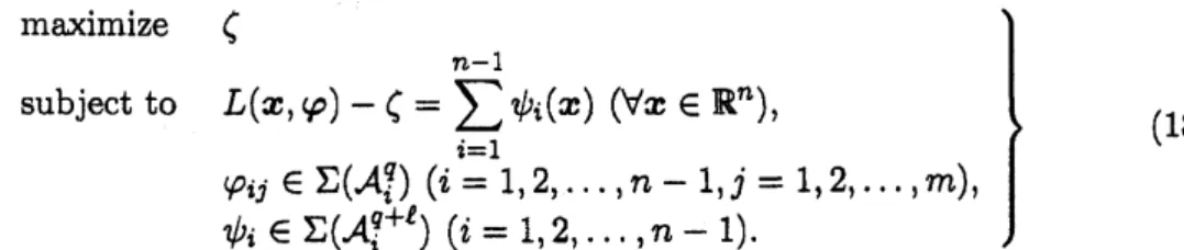
relaxation ofthePOP (15):

subject to $L$(x,$\varphi$) $- \zeta=\sum_{i=1}^{n-1}\psi_{\dot{\mathrm{t}}}(x)(\forall x\in \mathbb{R}^{n})$,

maximize

$\zeta\varphi_{ij}\in\Sigma(A_{i}^{q})(i=1,2, \ldots, n- 1, j=1,2, \ldots,m)$

,

$\}$ (18)

$\psi_{i}\in\Sigma(A_{t}^{q+\ell})(i=1,2, \ldots,n-1)$

.

It should be noted that the size ofevery support set in the SOS relaxation (18) is inde

pendent ofthe dimension $n$ of the POP (15). When $m$ and $q$ are fixed, the total size

ofsupport sets in the SOS relaxation (18) grows linearly with the dimension $n$ while the

growth rate of the total size ofsupport sets in the SOS relaxation (16)

as

well

as

that in

the SOS relaxation (17) are of $O(n^{q+\ell})$

.

This shows that the SOS relaxation (18) has

a

considerable computational advantage in solving the

POP

(15) with large dimension $n$

.

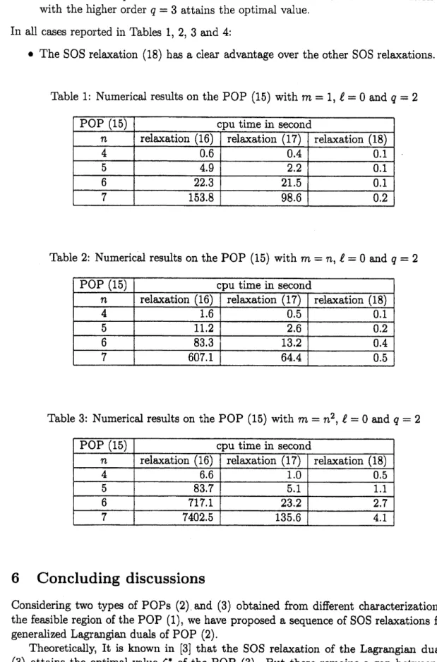
The numerical experiment

was

done using SDPA 6.0 [10]

on

Pentium IV (XEON) 2.4 GHz with $6\mathrm{G}\mathrm{B}$ memory, and the optimal values of the POP (15) with $m\in\{1, n, n^{2}\}$, $\ell\in\{1,3\}$, and $n\in\{4,5,6,7\}$

were

computed byGloptiPoly [2]. Tables 1, 2 azxd3 show

some numerical results from the three SOS relaxations (16), (17) and (18) of the POP

(15) with $m\in\{1, n, n^{2}\}$, $\ell=1$ aaxd dimension _{$n\in\{4,5,6,7\}$}

.

We observe that:

.

All the SOS relaxations (16), (17) and (18) attain optimal values of the POP (15)

with the lowest order $q=2.$

$\mathrm{o}$ The SOS relaxation (17) requires less cpu time than the SOS relaxation (16), and

the difference in cpu time becomes larger

as

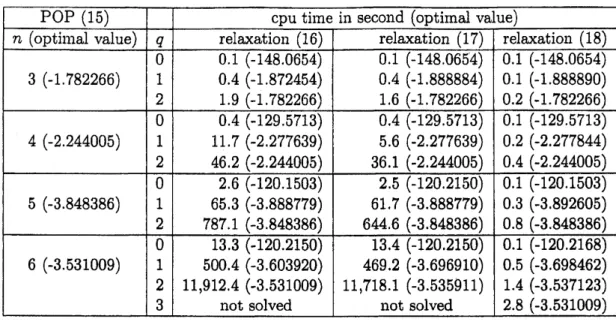
$m$ increases.

Table

4

shows

some

numerical results ffom the three

SOS

relaxations (16), (17) aatd (18)

of the

POP

(15) with $m=n$, $P=3$ and_dimension $n\in\{3,4,5,6\}$

.

In this

case:

o The SOS relaxations (17) aaxd (18) attain optimal values of the POP (15)

or

their

lower bounds of(almost) the

same

quality as the SOS relaxation (16).

$\circ$ The SOS relaxation (17) requires less cpu time than the SOS relaxation (16), but

the difference is small.

$\mathrm{o}$ When$n=6,$ theSOS relaxation (16) withtheorder$q=2$ attainsthe optimalvalue,

98

bounds for the optimal value. It should also be noted that the SOS relaxation(18)

with thehigher order $q=3$ attains theoptimal value.

In all

cases

reported in Tables 1, 2, 3 alld 4:

$\mathrm{o}$ The

SOS

relaxation (18) has

a

clear advantage

over

the other SOS relaxations.

Table 1: Numerical results

on

the POP (15) with $m=1$

,

$\ell=0$ and_$q=2$

POP (15) $\mathrm{c}\mathrm{p}\mathrm{u}$time in second

$n$ relaxation (16) relaxation ($1\underline{7)}$ relaxation (18)

4 0.6 0.4 0.1 5 4.9 2.2 -0.1 $\overline{6}$ 22.3 21.5 0.1

7

153.8

98.6

0.2

Table 2: Numerical results

on

thePOP (15) with $m=n$,$\ell=0$ and _$q=2$

POP

(15) cpu time in second

$n$ relaxation (16) relaxation (17) relaxation 18)

4 1.6 0.5 0.1

5 $\overline{11}$

.2–

2.6 0.2

683.3

13.2

0.4

7

607.1

64.4

0.5

Table 3: Numerical results

on

the POP (15) with $m=n^{2}$, $\ell=0$ and _$q=2$

$\mathrm{P}\mathrm{O}\underline{\mathrm{P}}(15)$ cpu time in second

$n$ relaxation (16) relaxation (17) relaxation (18)

4 6.6 1.0 0.5 5 83.7 5.1 1.1 6 – 717.1 $2\underline{3}$

.2-2.7

7 7402.5 135.6 – 4.1

6

Concluding

discussions

Considering two types of POPs (2) and (3) obtained from different characterizations of

the feasibleregion ofthe POP (1),

we

have proposed

a

sequence of SOS relaxations from

generalized Lagraiigian duals of POP (2).

Theoretically, It is known in [3] that the SOS relaxation of the Lagraiigian dual of

$\mathrm{e}\mathrm{e}$

Table 4: Numerical results on thePOP (15) with $m=n$ and $\ell=3$

POP (15) cpu time in second (optimal value)

$n$ (optimal value) $q$ relaxation (16)

– relaxation (17) relaxation (18) 00.1 (-148.0654) 0.1 (-148.0654) $0.\overline{1}$(-148.0654) 3 (-1.782266) 10.4 (-1.872454) 0.4 (-1.888884) 0.1 (-1.888890) 21.9 (-1.782266) $1.6(-$-1.782266$)$ $0.2_{-}(- 1.782266)$ 00.4 (-129.5713)

–0.4

(-129.5713) 0.1 (-129.5713) 4 (-2.244005) 111.7 (-2.277639)

5.6

(-2.277639) 0.2 (-2.277844) 2

46.2

(-2.244005)

36.1

(-2.244005) $0\underline{.4}$ $(- 2.244005)$

02.6

(-120.1503) 2.5 (-120.2150) 0.1 (-120.1503) 5 (-3.848386) 1 65.3 (-3.888779) 61.7 (-3.888779) 0.3 (-3.892605) 2787.1 (-3.848386) 644.6 (-3.848386) 0.8 (-3.848386)

013.3

(-120.2150) 13.4 $(- 120.2\overline{1}50)$ 0.1 (-120.2168) 6 (-3.531009) 1 500.4 (-3.603920)

469.2

(-3.696910) 0.5 (-3.698462) 211,912.4 (-3.531009) 11,718.1 (-3.535911) 1.4 (-3.537123)

3not solved not solved 2.8 (-3.531009)

Lagrangian dual of(2) alld its SOSrelaxation in Section 4.2; the former attains(’but the

latter is not guaranteed to attain $\zeta^{*}$

.

Thus it is interesting to prove or disprove that the

SOS relaxation ofthe Lagrangian dual of (2) attains $\mathrm{s}*$

.

This will be

a

subject of future

study.

The size of the

SOS

relaxation

or

the SDP relaxation obtained from the Lagrangian

dualapproach byexploiting sparsity is smallerthan the size of Lasserre’s SDP relaxation.

This is of

course

a nice feature, but this may not necessarily

mean

that the former SDP

relaxation is

as

effective

as

the latter in practice. To attain an approximation to the

optimal value $\langle$’ of the POP (1) with as high accuracy

as

the one from Lasserre’s SDP

relaxation, we may need higher degree SOS polynomials in our dual approach, which

makes the size of the resultingSDP relaxation larger.

One of the advantages of the proposed method is that we have much flexibility in

implementation of the SOS relaxation and the SDP relaxation of the POP (1); sets of

Lagrangian multiplier

SOS

polynomials satisfying the assumption of Theorem 3.1

can

be

freely chosen to strengthen the resulting relaxations. We have presented all illustrative

example of how the framework of the proposed

SOS

relaxation

can

be used to have

a

practical

SOS

relaxation exploitingastructured sparsity. Numerical resultsofthe example

have indicated that it is possible to drastically improve computational efficiency of SOS

relaxations bymaking proper heuristic choices of supports, depending

on

problems.

Additionalnumerical experiments

on

theSDPrelaxation with heuristicaly chosen

sup-ports

were

performedfor various types ofpolynomial optimization problems with certain

types of sparsity. We have not included the numerical results from the additional

nu-merical experiments in this paper because

we

believe that the discussion of heuristics is

beyond the scope ofthis paper. The main purposeofthis paperhas been proposing

gen-eral methodsfor sparsity in SDP relaxations forpolynomial optimization and introducing

Lagrangian dual and penalty function approaches into SDP relaxations for polynomial

relax-100

ations could improve the efficiency, it would be

necessary

to address issues such as (i)

a

reasonable

definition

of structured sparsity in polynomial optimization problems, (ii)

technical details of heuristic choices of supports, and (iii) extensivenumericalexperiments

on various problems with structured sparsity. These will consist ofa paper

on

practical

performance ofthe heuristics, which we hope to present in

near

future.

References

[1] M. D. Choi, T. Y. Lam, and B. Reznick, “Sums of squares of real polynomials”,

Proceedings

_of

Symp.o

sia in Pure Mathematics, 582 (1995)

103-126.

[2] D. Henrion and J. B. Lasserre, ”GloptiPoly: Global optimization

over

polynomials

with Matlab andSeDuM\"i, Laboratoire d ’_{Analyseet d}’

Architecture des Syst‘emes,

Centre National de la Recherche Scientiflque, 7 Avenue du Colonel Roche,

31077

Toulouse, cedex 4, Prance, February2002.

[3] S. Kim, M. Kojima and H. Waki, “GeneralizedLagr angian duals axxdsumsofsquares

relaxations of $\mathrm{s}\mathrm{p}\mathrm{a}\mathrm{r}\mathrm{s}\dot{\mathrm{e}}$ polynomial optimization problems, Research Report B-395,

Dept. of Mathematical and computing Sciences, Tokyo Institute of Technology,

Me-guro, Tokyo 152-8552, September2003. Revised July2004. Toappear in SIAM

Jour-nal

on

Optimization.

[4] M. Kojima,

S.

Kim and H. Waki, “A generalframework for convex relaxation of

poly-nomial optimization problems

over

cones”, Journal

_of

Operations Research Society

of

Japan, 462 (2003) 125-144.

[5] M. Kojima, S. Kim and H. Waki, “Sparsity in

sums

of squares of polynomials”,

Re-search ReportB-391, Dept.ofMathematical andcomputing Sciences, Tokyo Institute

of Technology, Meguro, Tokyo 152-8552, June

2003.

Revised August 2003. To appear

in Mathematical Programming.

[6] J. B. Lasserre, “Globaloptimizationwithpolynomials and the problems of moments”,

SIAM Journal on Optimization, 11 (2001) 796-817.

[7] P. A. Parrilo, “Semidefinite programming relaxations for semialgebraic problems”,

Mathematical Programming, 96 (2003) 293-320.

[8] V. Powers andT. W\"ormann, “An algorithm for

sums

ofsquares of real polynomials”

,

Journal

of

Pure and Applied Algebra, 127 (1998)

99-104.

[9] B. Reznick, “Extremal psd forms with few terms”, Duke Mathematical Journal, 45

(1978) 363-374.

[10] M. Yamashita, K. Pujisawa and M. Kojima, “Implementation aaxd evaluation of

SDPA 6.0 (SemiDefifinite Programming Algorithm 6.0)”, Optimization Methods and