NUMERICAL
REAL INVERSION
FORMULAS OF
THE
LAPLACE
TRANSFORM
BY
USING
THE SINC
FUNCTIONS
T.
MATSUURA
(
松浦勉
),
A.
AL-SHUAIBI, H.
FUJIWARA
(
藤原宏志
),
S.
SAITOH
(
齋藤三郎
) and M.
SUGIHARA
(
杉原正顕)
Abstract
We
shall givea very
natural and numerical real inversionformula
ofthe Laplace transform for general $L_{2}$ data following the ideas of best
approximations, generalized inverses, theTikhonov regularization and
the theory of reproducing kernels. Furthermore,
we
shall additionallyuse
theSinc
functions (theSinc
method) toour
general theory, tosolve the related integral equation. However, the
new
method in thispaper
for the real inversion formula will be reduced to the solutionof linear simultaneous equations. This real inversion formula
may
be expected to be practical to calculate the inverses of the Laplace
transform
by computers when the realdata
contain noise
or
errors.
We shall illustrate examples and justify
our
computational work.1
Introduction
We shall give
a
very natural and numerical real inversion formula ofthe Laplace transform
$\underline{(\mathcal{L}F)(p)=f(}p)=\int_{0}^{\infty}e^{-pt}F(t)dt$, $P>0$ (1.1)
’2000 Mathematics Subject Classification: Primary $44A15,35K05$, 30C40 Key words and phrases: Laplace transform, real inversion, numerical inversion, reproducing kernel, Tikhonov regularization, Sobolev space, approximate inverse, sinc method, sampling
the-orem
forfunctions $F$of
some
natural functionspace. This integral transformis, ofcourse, very fundamental in mathematical science. The inversion
of the Laplace transform is, in general, given by
a
complex form,however,
we
are
interested in andare
requested to obtain its realinversion in many practical problems. However, the real inversion
will be very involved and
one
might think that its real inversion willbe essentialy involved, because
we
must catch “analyticity” from thereal
or
discrete data. Note that the image functions of the Laplacetransform
are
analyticon
some
half complex plane. For complexityof the real
inversion formula
of the Laplace transform,we
recall, forexample, the following formulas:
$\lim_{narrow\infty}\frac{(-1)^{n}}{n!}(\frac{n}{t})^{n+1}f^{(n)}(\frac{n}{t})=F(t)$
(Post [15] and Widder [27,28]), and
$\lim_{narrow\infty}\Pi_{k=1}^{n}(1+\frac{t}{k}\frac{d}{dt})[\frac{n}{t}f(\frac{n}{t})]=F(t)$,
([27,28]).
Furthermore,
see
[1-8,16,17,21,25,26,28,29]
and the recent relatedarticles [10] and [11].
See
ako the greatreferences
$[29,30]$.
Theprob-lem
may
be related to analytic extension problems,see
[11] and [22].In this
paper,
we
shall givea new
type andvery
natural real inversionformula from the viewpoints of best approximations, generalized
in-verses
and the Tikhonov regularization by combining thesefundamen-tal ideas and methods by
means
ofthe theory ofreproducing kernels.Furthermore,
we
shalluse
the sinc functions (the sinc method)as
a
new
approarch to solve the crucial Fredholm integral equation of thesecond kind
on
the half space inour
general theory. We shall alsopropose
a
new
method for the real inversion of the Laplace transformbased essentially
on
linear simultaneous equations. Wemay
think thatthis real
inversion formula
is practical and natural.Error
analysis willbe also considered.
2
Background General Theorems
Let $E$ be
an
arbitrary set, and let $H_{K}$ bea
reproducing kernel Hilbertany
Hilbertspace
$\mathcal{H}$we
considera
bounded linear operator $L$ from$H_{K}$ into $\mathcal{H}$
.
Weare
generally interested in the best approximationproblem
$\inf_{f\in H_{K}}\Vert Lf-d\Vert_{\mathcal{H}}$ (2.2)
for a vector $d$ in $\mathcal{H}$
.
However, this extremal problem is quite involvedin existence and representation. See [16,19,20] for the details.
Now, for the Tikhonov regularization,
we
set, for any fixed positive$\alpha>0$
$K_{L}(\cdot,p;\alpha)=(L^{*}L+\alpha I)^{-1}K(\cdot,p)$,
where $L^{*}$ denotes the adjoint operator of$L$
.
Then, by introducing theinner product
$(f,g)_{H_{K}(L;\alpha)}=\alpha(f,g)_{H_{K}}+(Lf, Lg)_{\mathcal{H}}$, (2.3)
we
shall construct the Hilbert space $H_{K}(L;\alpha)$ comprising functions of$H_{K}$
.
Thisspace, of course, admitsa
reproducing kernel. FMrthermore,we
dirctly obtainProposition 2.1 (/18-20]) The extremal
function
$f_{d,\alpha}(\rho)$ in the Tikhonovregularization
$\inf_{f\in K}\{\alpha||f||_{H_{K}}^{2}+\Vert d-Lf\Vert_{?t}^{2}\}$ (2.4)
exists uniquely and it is represented in terms
of
the kemel $K_{L}(p, q;\alpha)$$by$:
$f_{d,\alpha}(p)=(d, LK_{L}(\cdot,p;\alpha))_{\mathcal{H}}$ (2.5)
where the kemel $K_{L}(p, q;\alpha)$ is the reproducing kemel
for
the Hilbertspace $H_{K}(L;\alpha)$ and it is determined as the unique solution $\tilde{K}(p, q;\alpha)$
of
the equation:$\tilde{K}(p, q;\alpha)+\frac{1}{\alpha}(L\tilde{K}_{q}, LK_{p})_{\mathcal{H}}=\frac{1}{\alpha}K(p, q)$ (2.6)
with
$\tilde{K}_{q}=\tilde{K}(\cdot, q;\alpha)\in H_{K}$
for
$q\in E$, (2.7)and
In (2.5), when $d$ contains
errors
or noise,we
need itserror
estimate.For this, we
can
use the general result:Proposition 2.2 (/14]). In (2.5),
we
have the estimate$|f_{d,\alpha}(p)| \leq\frac{1}{\sqrt{\alpha}}\sqrt{K(p,p)}\Vert d\Vert_{\mathcal{H}}$
.
For
theconvergence
rateor
the results for noisy data,see,
([9]).3
A Natural
Situation
for Real
Inver-sion
Formulas
In order to apply the general theory in Section 2 to the real
inver-sion formula
of the Laplace transform,we
shall recal the “naturalsituation” based
on
[17].We shall
introduce
the simple reproducing kemel Hilbertspace
(RKHS) $H_{K}$ comprised of absolutely continuous functions $F$
on
thepositive real line $R^{+}$ with finite
norms
$\{\int_{0}^{\infty}|F’(t)|^{2}\frac{1}{t}e^{t}dt\}^{1/2}$
and satisfying $F(O)=0$
.
This Hilbert space admits the reproducingkernel $K(t, t’)$
$K(t, t’)= \int_{0}^{\min(t,t’)}\xi e^{-\xi}d\xi$ (3.8)
$=\{\begin{array}{llll}-te^{-t}- e^{-t}+1 for t\leq t’-t’e^{-t’} -e^{-t}’+1 for t\geq t\end{array}\}$
(see [16],
pages
55-56). Thenwe
see
that$\int_{0}^{\infty}|(\mathcal{L}F)(p)p|^{2}dp\leq\frac{1}{2}||F||_{H_{K}}^{2}$; (3.9)
that is, the linear operator
$(\mathcal{L}F)(p)p$
on
$H_{K}$ into $L_{2}(R^{+}, dp)=L_{2}(R^{+})$ is bounded. For the reproducingspaces ([17]). Therefore, from the general theory in
Section
2,we
obtain
Proposition 3.1 $(l^{15}7)$
.
For any$g\in L_{2}(R^{+})$ andfor
any $\alpha>0$, thebest approximation $F_{\alpha,g}^{*}$ in the $8ense$
$\inf_{F\in H_{K}}\{\alpha\int_{0}^{\infty}|F’(t)|^{2}\frac{1}{t}e^{t}dt+\Vert(\mathcal{L}F)(p)p-g||_{L_{2}(R+}^{2})\}$
$= \alpha\int_{0}^{\infty}|F_{\alpha,g}^{*l}(t)|^{2}\frac{1}{t}e^{t}dt+||(\mathcal{L}F_{\alpha,g}^{*})(p)p-g\Vert_{L_{2}(R^{+})}^{2}$ (3.10)
exists uniquely and
we
obtain the representation$F_{\alpha,g}^{*}(t)= \int_{0}^{\infty}g(\xi)(\mathcal{L}K_{\alpha}(\cdot,t))(\xi)\xi d\xi$
.
(3.11)Here, $K_{\alpha}(\cdot, t)$ is determined by the
functional
equation$K_{\alpha}(t, t’)= \frac{1}{\alpha}K(t,t’)-\frac{1}{\alpha}((\mathcal{L}K_{\alpha,t’})(p)p, (\mathcal{L}K_{t})(p)p)_{L_{2}(R+})$ (3.12)
for
$K_{\alpha,t’}=K_{a}(\cdot, t’)$
and
$K_{t}=K(\cdot,t)$
.
4
Sampling
Theory
and Reproducing
Kernels
In order to solve the integral equation (3.11), numerically,
we
shallemploy the sinc method. At first
we
$shaU$ fix notations and basicresults in the sampling theory following the book by F. Stenger[23]
and at the
same
timewe
shall show the basic relation of the samplingtheory and the theory of reproducing kernels.
We shall consider the integral transform, for
a
function
$g$ in$f(z)= \frac{1}{2\pi}\int_{-\pi/h}^{\pi/h}g(t)e^{-izt}dt$
.
(4.13)In order to identify the image
space
following thetheoryofreproducingkernels
[16],we
form the reproducing kernel$K_{h}(z, \overline{u})=\frac{1}{2\pi}\int_{-\pi/h}^{\pi/h}e^{-izt}\overline{e^{-iut}}dt$ (4.14)
$= \frac{1}{\pi(z-\overline{u})}\sin\frac{\pi}{h}(z-\overline{u})$
$:= \frac{1}{h}$Sinc $( \frac{z-\overline{u}}{h})$
$:= \frac{1}{h}S(k, h)(z-\overline{u}+hk)$
,
by the notations in [23]. The image space of (4.13) is called the
Paley-Wiener space $W( \frac{\pi}{h})$ comprised of all analytic functions ofexponential
type $satis\theta ing$
,
forsome
constant $C$ andas
$zarrow\infty$$|f(z)|\leq C$exp $( \frac{\pi|z|}{h})$
and
$\int_{R}|f(x)|^{2}dx<\infty$
.
From
the identity$K_{h}(jh,j’h)= \frac{1}{h}\delta(j,j’)$
(the Kronecker’s $\delta$), since
$\delta(j,j’)$ is the reproducing kemel for the
Hilbert space $\ell^{2}$, from
the general theory of integral transforms and
the Parseval’s identity
we
have the isometric identities in (4.13)$\frac{1}{2\pi}\int_{-\pi/h}^{\pi/h}|g(t)|^{2}dt$
$=h \sum_{j}|f(jh)|^{2}$
That is, the reproducing kernel Hilbert space $H_{K_{h}}$ with $K_{h}$($z$,Of) is
characterized
as a
space comprising the Paley-Wiener space $W( \frac{\pi}{h})$and with the
norm
squares
above. Herewe
used the well-known resultthat $\{jh)\}_{j}$
is
a
unique set for the Paley-Wienerspace
$W( \frac{\pi}{h})$; that is,$f(jh)=0$ for all $j$ implies $f\equiv 0$
.
Then, the reproducing property of$K_{h}(z,\overline{u})$ states that
$f(x)= \langle f(\cdot), K_{h}(\cdot, x)\rangle_{H_{K_{h}}}=h\sum_{j}f(jh)K_{h}(jh, x)$
$= \int_{R}f(\xi)K_{h}(\xi,x)d\xi$
.
In particular,
on
the real line $x$,
this representation is the samplingtheorem which represents the whole data $f(x)$ in terms of the discrete
data $\{f(jh)\}_{j}$
.
Fora
general theory for the sampling theory anderror
estimates for
some
finite points $\{hj\}_{j}$,
see
[16].5
New Algorithm
By setting
$(\mathcal{L}K_{\alpha}(\cdot, t))(\xi)\xi=H_{\alpha}(\xi,t)$,
which is needed in (3.11),
we
obtain the Fredholm integral equationof the second type
$\alpha H_{\alpha}(\xi, t)+\int_{0}^{\infty}H_{\alpha}(p,t)\frac{1}{(p+\xi+1)^{2}}dp$
$=f( \xi, t)=-\frac{e^{-t\xi}e^{-t}}{\xi+1}(t+\frac{1}{\xi+1})+\frac{1}{(\xi+1)^{2}}$
.
(5.15)We shall
use
the double exponential transform $f_{0}n_{oW}ing$ the idea [24]$\xi=\phi(x)=\exp$($\frac{\pi}{2}$ sinh$x$),
$\phi’(x)=\frac{\pi}{2}$ cosh$x\exp$($\frac{\pi}{2}$ sinh$x$).
Note that this$\phi(x)$ is
a
monotonically increasing functionand $\phi(-\infty)=$$0$ and $\phi(\infty)=\infty$
.
In addition, for examplesand
$\phi(16)=5.860\cross 10^{3030999}$
.
So there is
no
need for settingso
wide interval of integration froma
practical point of view.
Then,
we
have$H_{\alpha}(\xi,t)=H_{\alpha}(\phi(x),t)=\tilde{H}_{\alpha}(x, t)$
and so,
$\tilde{H}_{\alpha}(x, t)=\sum_{j_{=-\infty}}^{j=\infty}\tilde{H}_{\alpha}(jh, t)Sinc(\frac{x}{h}-j)$
and
$\alpha\tilde{H}_{\alpha}(x,t)$
$+ \int_{-\infty}^{\infty}\tilde{H}_{\alpha}(z, t)\frac{1}{(\phi(z)+\phi(x)+1)^{2}}\phi^{j}(z)dz=f(\phi(x), t)$
.
(5.16)We
shall approximateas
follows:$\tilde{H}_{\alpha}(x,t)\simeq\sum_{j=-N}^{j=N}\tilde{H}_{\alpha}(jh, t)Sinc(\frac{x}{h}-j)$
.
For
error
estimates forsome
finite points $\{hj\}_{j}$,
see
[16]. Then,we
have
$\alpha\sum_{j}\tilde{H}_{\alpha}(jh,t)Sinc(\frac{x}{h}-j)$
$+ \int_{-\infty}^{\infty}\sum_{k}\tilde{H}_{\alpha}(kh, t)Sinc(\frac{z}{h}-k)\frac{1}{(\phi(z)+\phi(x)+1)^{2}}\phi’(z)dz=f(\phi(x),t)$
.
(5.17)
Rom the identities
$\int_{-\infty}^{\infty}Sinc(\frac{x}{h}-i)Sinc(\frac{x}{h}-j)dx=h\delta_{ij}$
and
$\int_{-\infty}^{\infty}\frac{1}{(\phi(z)+\phi(x)+1)^{2}}Sinc(\frac{x}{h}-l)dx=\frac{1}{(\phi(z)+\phi(lh)+1)^{2}}h$
,
by setting
we
obtain the equation$\alpha\tilde{H}_{\alpha}(lh, t)+\sum_{k}\tilde{H}_{\alpha}(kh, t)A_{lk}=f(\phi(lh), t)\equiv f(lh, t)$ (5.18)
and the representation
$F^{*}(t)= \int_{0}^{\infty}g(\xi)H_{\alpha}(\xi,t)d\xi=\int_{-\infty}^{\infty}g(\phi(x))H_{\alpha}(\phi(x),t)\phi’(x)dx$
$\simeq h\sum_{i}g(\phi(ih))\tilde{H}_{\alpha}(ih,t)\phi’(ih)$
.
6
Inverses for
More General
FUnctions
As
one
ofthe main features ofour
method,we
can
easily generalize theapproximation function space. By
a
suitable transform,our
inversionformula in
Section 5
is applicable formore
general functionsas
follows:We
assume
that $F$ satisfies the properties (P):$F\in C^{1}[0, \infty)$
,
$F’(t)=o(e^{\alpha t})$, $0< \alpha<k-\frac{1}{2}$
,
and
$F(t)=o(e^{\beta t})$
,
$0<\beta<k$ 一 $\frac{1}{2}$Then, the function
$G(t)=\{F(t)-F(O)-tF’(0)\}e^{-kt}$ (6.19)
belongs to $H_{K}$
.
Then,$( \mathcal{L}G)(p)=f(p+k)-\frac{F(0)}{p+k}-\frac{F’(0)}{(p+k)^{2}}$
.
(6.20)Therefore, if
we
know $F(O)$ and $F’(O)$,
then from$g(p)=(\mathcal{L}G)(p)$
by the method in Section 5, we obtain $G(t)$ and so, $hom$ the identity
$F(t)=G(t)e^{kt}+F(0)+tF’(0)$ (6.21)
we
have the inverse $F(t)hom$ the data $f(p),$$F(O)$ and $F’(O)$ through7
Numerical
Experiments
We used $h=0.05$ and for $t$
,
we take the span with0.01.
For thesimultaneous equations (5.18), we take from $\ell=-200$ to $\ell=799$;
that is,
1000
equations. We solved such equations for $[0,4.99]$ withthe span
0.01
for $t$.
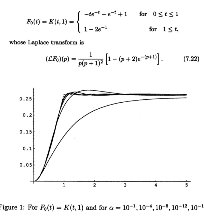
We shall give
a
numerical experiment for the typical example$F_{0}(t)=K(t, 1)=\{\begin{array}{ll}\text{一} te^{-t}-e^{-t}+1 for 0\leq t\leq 11-2e^{-1} for 1\leq t,\end{array}$
whose Laplace transform is
$( \mathcal{L}F_{0})(p)=\frac{1}{p(p+1)^{2}}[1-(p+2)e^{-(p+1)]}$
.
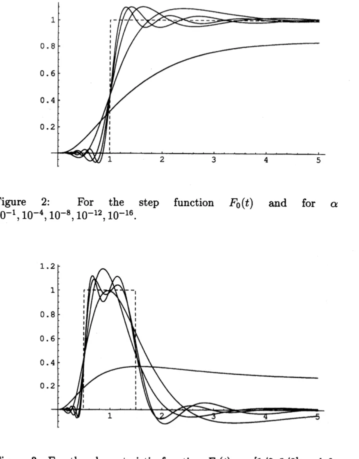
(7.22)Figure
2:
For
the
step
$10^{-1},10^{-4},10^{-8},10^{-12},10^{-16}$
.
function
$F_{0}(t)$and
for
$\alpha$Figure
3:
For the characteristic
function
$F_{0}(t)$on
[1/2, 3/2] and for
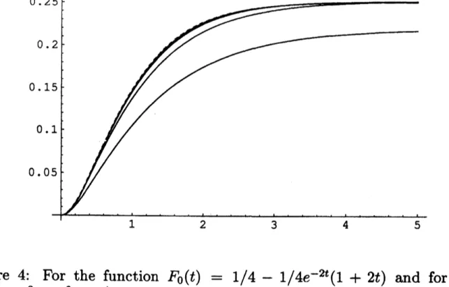
$\alpha=$Figure 4: For the
function
$F_{0}(t)=1/4-1/4e^{-2t}(1+2t)$and for
$\alpha=$ $10^{-1},10^{-2},10^{-3},10^{-4}$.
Acknowledgements
Al-Shuaibi
visitingGunma
Universitywas
supported by the JapanCooperation Center, Petroleum, the Japan Petroleum
Institute
(JPI)and King Fahd University of Petroleum and Minerals, and he wishes
to express his deep thanks Professor
Saburou
Saitoh and Mr. HidekiKonishi of
the
JPI for their kind hospitality. S. Saitoh is $s$upported inpart by the
Grant-in-Aid
for Scientific Research (C)(2)(No. 16540137;No. 19540164) from the Japan Society for the Promotion
Science.
S.Saitoh and T. Matsuura
are
partially supported by the MitsubishiFoundation, the 36th, Natural Sciences, No.
20
(2005-2006).References
[1] Abdulaziz Al-Shuaibi, On the inversion
of
the Laplacetransform
by
use
of
a
regularized displacement opera$tor$,
Inverse Problems,13(1997),
1153-1160.
[2] Abdulaziz Al-Shuaibi, The
Riemann
zetafunction
used in the[3]
Abdulaziz
Al-Shuaibi,Inversion
of
the Laplacetransform
viaPost- Widder formula, Integral Transforms and Special Functions,
11(2001),
225-232.
[4] K. Amano, S. Saitoh and A. Syarif, A Real Inversion Fomula
for
the Laplace $\pi_{ansform}$ in a Sobolev Space, Z. Anal. Anw. 18(1999),
1031-1038.
[5] K. Amano,
S.
Saitoh and M. Yamamoto, Errorestimatesof
the real$inver8ion$
fomulas
of
the Laplace transform, Integral Transformsand Special Functions, 10(2000),
165-178.
[6]
A. Boumenir and A.
Al-Shuaibi, The Inverse Laplace $\pi_{ansform}$and Analytic
Pseudo-Differential
$0perator8$,
J.
Math.Anal.
Appl. 228(1998),
16-36.
[7]
D.-W.
ByunandS.
Saitoh,A
realinversionfomula
for
the Laplacetransform, Z.
Anal. Anw.
12(1993),597-603.
[8]
G.
Doetsch, Handbuch der Laplace $?$}$nnsformation$, Vol. 1.,Birkhaeuser Verlag, Basel,
1950.
[9] H. W. Engl, M. Hanke and A. Neubauer, Regularization ofInverse
Problems, Mathematics and Its Applications, 376(2000), Kluwer
Academic
Publishers.[10] V. V. Kryzhniy, Regularized $Inver8ion$
of
Integral $\pi ansforma-$tions
of
MellinConvolution
$\Phi^{pe}$,
Inverse Problems, 19(2003),1227-1240.
[11] V. V. Kryzhniy, Numerical inversion
of
the Laplacetransform:
analysis via regularized analytic continuation, Inverse Problems,
22(2006),
579-597.
[12] T. Matsuura and
S.
Saitoh, Analytical and numerical solutionsof
linear ordinarydifferential
equations withconstant
coefficients,Journal
of
Analysis andApplications,
3(2005),pp.
1-17.
[13] T. Matsuura and
S.
Saitoh, Analytical and numerical realin-version
formulas of
the Laplace transform, TheISAAC Catani
Congress
Proceedings (to appear).[14] T. Matsuura and
S.
Saitoh, Analytical and numencal inversionfomulas
in the $Gau88ian$ convolution by using the Paley- Wienerspaces, Applicable Analysis, 85(2006),
901-915.
[15] E. L. Post, Generalized diffentiation, ‘TMrans.
Amer.
Math.Soc.
[16] S. Saitoh, Integral Iansforms, Reproducing Kemels and their
Applications, Pitman Res. Notes in Math. Series 369, Addison
Wesley Longman Ltd (1997), UK.
[17]
S.
Saitoh, Approximate real inversionformulas
of
the Laplacetransform,
Far East
J. Math.Sci.
11(2003),53-64.
[18]
S.
Saitoh, Approximate Real Inversion Formulasof
theGaussian
Convolution, Applicable Analysis, 83(2004),
727-733.
[19] S. Saitoh, Best approximation, Tikhonov rtegularization and
re-producing $kernel_{8}$, Kodai. Math. J. 28(2005),
359-367.
[20]
S.
Saitoh, Tikhonov regulanzation and the theoryof
reproducingkemels, Proceedings of the 12th International Conference
on
Fi-nite
or
Infinite Dimensional Complex Analysis and Applications,Kyushyu
University Press
(2005),291-298.
[21]
S.
Saitoh,Vu Kim Tuan
and M. Yamamoto,Conditional
Stabilityof
a
RealInverse
Formulafor
the Laplace $\pi an8form$,
Z. Anal.Anw.
20(2001),193-202.
[22] S. Saitoh, N. Hayashi and M. Yamamoto (eds.), Analytic
Exten-sion Formulas and their Applications, (2001), Kluwer Academic
Publishers.
[23] F. Stenger, Numerical Methods Based
on Sinc
and Analytichnc-tions,
Springer Series
in Computational Mathematics, 20,1993.
[24] H. Ibkahasi and M. Mori, Double exponential
formulas for
nu-merical integration, Publ.
Res. Inst.
Math.Sci.
9(1974),511-524.
[25] Vu
Kim
Tuan and Dinh Thanh Duc,Convergence rate
of
Post-Widder appro rzmate
inversion
of
the Laplace transform, VietnamJ. Math. 28(2000),
93-96.
[26] VuKim
Tuan
and Dinh ThanhDuc, Anew
realinversionformula
for
the Laplacetransform
and its convergence rate, Frac. Cal.&
Appl. Anal. 5(2002),
387-394.
[27] D. V. Widder, The inversion
of
the Laplace integral and there-lated
moment
problem, hans.Amer.
Math.Soc.
36(1934),107-2000.
[28] D. V. Widder, The Laplace $\pi_{ansf_{07}m}$
,
Princeton University
Press,
Princeton, 1972.
[29] $http://librury.wolffam.com/inforoenter/MathSource/4738/$
T. Matsuura
Department ofMechanical System Engineering,
Graduate School of Engineering,
Gunma
University, Kiryu, 376-8515, JapanE-mail: [email protected]
Abdulaziz
Al-Shuaibi
KFUPM
Box 449, Dhahran 31261,Saudi
ArabiaE-mail: [email protected]
H. Fujiwara
Graduate School of Informatics,
Kyoto University, Japan
E-mail: fujiwara@acs.$i$.kyoto-u.ac.jp
S.
Saitoh
Department ofMathematics,
Graduate
School
of Engineering,Gunma
University, Kiryu, 376-8515, JapanE-mail: [email protected]
and M. Sugihara
Department of Computer Science and Engineering,
Graduate School of Engineering, University of Tokyo
Bunkyou-Ku, Hongou, 113-8656, Japan