Swaption
pricing:
A
Binomial
Approach
法政大学・工学部 浦谷 規 (Uratani Tadaehi)
Department of Industrial and System Engineering
EngineeringSchool ofHosei University
1
Introduction
The Libor market model and Swap market model
are
inconsistent with each other in that theycan
not be simultaneously descrIbed by $\log$-normal processes.The market quots the at-the-money caps in term of their Black implied volatilitiae. Rom
these,
one can
infer caplet volatilites. Caplet implied volatilities give information about thedistribution offorwardLibor. The market
seems
toassume
that it is $\log$-normal with volatility.At-the-money European swaptions
are
also quoted in term of their Black implied volatilitiaewhich $g\ddagger ve$ information about
distribution
of swap rate.The Black model pricing is assumed
that
forward
swap rate follows $\log$-normal distribution.The purpose of this paper is to build
an
arbitrage-hee lattice model for swaption, whichis consistent with Libor market model and which provides
an
implementation method for thetheoretical closed-form formula which is dlfficult to get numericIl solution. We furthermore
compare the aPproximations of swaptIon pricing between swap market model and binomial
lattice inthmretical and numerical aePect.
There are several papers on solving inconsistency of two market models. We can see the
swap volatility approximation by Libor volatility in Rebonate[5]
or
$Brigo[1]$.
These approachesare mainly to adjest the swap volatility by using Libor volatilty. Recently, however, Davis and
Mataix-Pastor[2] have shown the possibility of negative forward Libor rate from coexistence
of Libor market model and Swap market model. This negative forward Libor could give
us
arbitrage opportunity.
Our
approximation by lattice would make it possible to get arbitrageopportunity.
The rest of this Paperisorganized
as
follows. InSection2we
provide notation andintroduceLibor market model which is based
on
HJM model. In Section 3,we
derive European payerswaption price formula for
Gaussian
volatility. The formula is aweightedaverage
of discountbonds with Gaissian
distribution
weight. However, it isnot easy taek to findnumerical solutionoffunctionwhich satisfy positivity of swaption. In section 4,
we
propose the numerical methodto get asolution of this function by binomiallattice, which
uses
the change ofmeasure
techiquebased
on
Jamishidan [3]. In Section 5is devoted to numerical example of flat term structureof Libor and volatility. After providing Swap market model with European payer swaption
formula, we compare numerical values of $coeffice\ddagger ent$ for discount bonds in the portfolio of
bonds replicatingtheswap. Finally,
we
dlscuss the replicationstrategy for arbitrage and closingremarks.
2
Libor model
We
assume
HJM-model
fordiscoutedbond pricesofmaturity$T_{i},$ $\{B_{i}(t)\}_{0\leq t\leq T_{1}}$ under risk neutralmeasure
$Q$,where the time span is $\delta=t_{i+1}-t_{i}$,
for
$i=0,$ $\cdots,$$N-1$ . Let $r(t)$ be spot rate and $\sigma^{i}(t)$ bethe volatility ofdiscount bond. The bond price of maturity of$T_{i}$ at time $T_{m}$ is, for$t\leq T_{m}\leq T_{i}$
$B_{i}(T_{m})=B_{i}(t)$exp $( \int_{t}^{T_{m}}r(s)ds+\int^{T_{m}}\sigma^{i}(s)dW(s)-\frac{1}{2}\int^{T_{m}}|\sigma^{i}(s)|^{2}ds)$
,
(2.1)and for the bond price of maturity $T_{i+1}$ is
$B_{i+1}(T_{m})=B_{i+1}(t)$exp $( \int^{T_{m}}r(s)ds+\int^{T_{m}}\sigma^{1+1}(s)dW(s)-\frac{1}{2}\int^{T_{m}}|\sigma^{i+1}(s)|^{2}ds)$
.
(2.2)Let $L_{i}(t)$ be a forward Libor from $T_{i}$ to $T_{i+1}$, then the Libor process is defined
as
$L_{i}(t)= \delta^{-1}(\frac{B_{i}(t)}{B_{i+1}(t)}-1)$.Dividing (2.1) by (2.2) and from the
definition
of Liborwe
get$\frac{1+\delta L_{i}(T_{m})}{1+\delta L_{i}(t)}=\exp(\int_{t}^{T_{m}}[\sigma^{i}(s)-\sigma^{i+1}(s)]dW(s)-\frac{1}{2}\int^{T_{m}}[|\sigma^{i}(s)|^{2}-|\sigma^{i+1}(s)|^{2}]ds)$ (2.3)
In HJM-model the forward process of settlement time $T$ is modeled
as
$df_{T}(t)=\mu_{T}(t)dt+\sigma_{T}(t)dW(t)$
where $\sigma_{T}$ is the volatility of forward process $\{f_{T}(t)\}$
.
For the settlement time $T_{1}$we
write thevolatility$\sigma_{i}(t)$ instead of$\sigma_{T:}(t)$
.
Thebond price at $t$ of maturity$T$ in (2.1) divided by (2.2) andlet $B_{t}(t)=1$, then
$B_{T}(t)= \frac{B_{T}(0)}{B_{t}(0)}$ exp $( \int_{0}^{t}(\sigma^{T}(s)-\sigma^{t}(s))dW(s)-\frac{1}{2}\int_{0}^{t}(|\sigma^{T}(s)|^{2}-|\sigma^{t}(s)|^{2})ds)$
Forward rate is defined
as
$f_{T}(t)=-\Phi\partial$log$B_{T}(t)$ and then$df_{T}(t)= \sigma^{T}(t)\frac{\partial}{\partial T}\sigma^{T}(t)dt-\frac{\partial}{\partial T}\sigma^{T}.(t)dW(t)$
By It\^o’s division rule
$\frac{d(B_{i}(t)/B_{i+1}(t))}{B_{i}(t)/B_{i+1}(t)}=$ ($\sigma(t)$ 一$\sigma^{i+1}(t)$)$(dW(t)-\sigma^{i+1}(t)dt)$
Under the risk adjusted
measure
$Q^{i+1}$$\frac{dL_{i}(t)\delta}{1+\delta L_{i}(t)}=(\sigma^{i}(t)-\sigma^{i+1}(t))dW^{i+1}(t)$,
when we define the risk adjested Measure $Q^{i+1}$ by $dQ^{i+1}/dQ= \mathcal{E}(\int_{0}^{T_{i+1}}\sigma^{i+1}(t)dW(t))$
,
then$W^{i+1}(t)=W(t)- \int_{0}^{t}\sigma^{i+1}(s)ds$is Brownian motion under $Q^{i+1}$ where $\mathcal{E}(\cdot)$ is stochastic
expo-nential.
Therefor Libor $L_{i}(t)$ is $Q^{i+1}$-martingale as,
The Bond Volatility $\sigma^{T}(t)=-\int_{t}^{T}\sigma_{s}(t)ds$ and let $v_{i}(t)$ be the volatility of Libor $L_{i}(t)$ ;
$v_{i}(t)= \sigma^{i}(t)-\sigma^{i+1}(t)=-\int^{T_{i}}\sigma_{u}(t)du+\int^{T_{i+1}}\sigma_{u}(t)du=\int_{T}^{T_{i+1}}\sigma_{u}(t)du$
In section 4 of binomial lattice model we
assume
$v_{i}$ is constant for $(T_{i}, T_{i+1})$ and in numericalexperiment section 5
assume a
constant $v=v_{i},$ $\forall i$.
Libor process isexpressed under$Q^{i+1}$ from(2.3)
as
follows,$L_{i}(T_{m})= \delta^{-1}(1+\delta L_{i}(t))\exp\{\int^{T_{m}}v_{i}(s)dW^{i+1}(s)-\frac{1}{2}\int^{T_{m}}|v^{i}(s)|^{2}ds\}-1$
3
Swaption
price of
Gaussian
volatility
The
payer
swaption is the option with strikeswap
rate $k$ and the maturity $T_{n}$, where theunderlying swap contract starts from $T_{n}$ to $T_{N}$ and payment period $\delta=T_{i}-T_{i-1}$, $i=$ $n+1,$$\cdots,$$N$
.
The payment at the maturity is$A(T_{n})= \max(B_{n}(T_{n})-B_{N}(T_{n})-k\delta\sum_{i=n+1}^{N}B_{i}(T_{n}), 0)$
where, $B_{i}(T_{j})$
denotes
the prioe at $T_{j}$ of bond of maturity time $T_{i}$.
The bond price of maturity $T_{n}$ is
1
at time $T_{n}$ then $A(T_{n})= \max(1-V(T_{n}),0)$ isa
putoption
on
bonds portfolio, where$V(T_{n})=B_{N}(T_{n})+k \delta\sum_{i=n+1}^{N}B_{i}(T_{n})$
Under risk neutral
measure
$Q$, the price ofswaption at time $0$is.
$S( O)=E^{Q}[\exp\{-\int_{0}^{T_{n}}r(s)ds\}A(T_{n})]$
Theorem
1 The swaption price ofGaussian
volatility HJM model is givenas
follows,$S( O)=B_{n}(0)N(d_{n})-B_{N}(0)N(d_{N})-k\delta\sum_{i=n+1}^{N}B_{i}(0)N(d_{i})$ (31)
where $d_{i}=d_{n}- \int_{0}^{T_{n}}(\sigma^{i}(s)-\sigma^{n}(s))ds$, $i=n+1,$
$\cdots,$$N$ and $d_{n}$ is the solution of equation;
$f(x)$ $=$ $\frac{B_{N}(0)}{B_{n}(0)}$
exn
$\{v(O,T_{n}, T_{N})\sqrt{T_{n}}x-\frac{1}{2}v(0,T_{n},T_{N})^{2}T_{n}$$+$ $k \delta\sum_{i=n+1}^{N}\frac{B_{1}(0)}{B_{n}(0)}$
exn
$\{v(0,T_{n},T_{i})\sqrt{T_{n}}x-\frac{1}{2}v(0,T_{n},T_{i})^{2}T_{n}\}-1=0$ (3.2)Proof.
Taking $B_{n}(t)$as
the numeraire for the payoff at time $T_{n}$;$\frac{V(T_{n})-1}{B_{n}(T_{n})}$ $=$ $\frac{B_{N}(0)}{B_{n}(0)}\exp\{\int_{0}^{T_{n}}(\sigma^{N}(t)-\sigma^{n}(t))dW^{n}(t)-\frac{1}{2}\int_{0}^{T_{n}}|\sigma^{N}(t)-\sigma^{n}(t)|^{2}dt$
$+$ $k \delta\sum_{i=n+1}^{N}\frac{B_{i}(0)}{B_{n}(0)}\exp$
{
$\int_{0}^{T_{n}}(\sigma^{i}(t)-\sigma^{n}(t))dW^{n}(t)$ 一 $\frac{1}{2}\int_{0}^{T_{n}}|\sigma^{i}(t)-\sigma^{n}(t)|^{2}dt$}
$-1$Let $U_{n}$ be
a
standarad normaldistributed variate, i.e. $U_{n}\sim N(0,1)$ anddefine the function;$f(U_{n})$ $=$ $\frac{B_{N}(0)}{B_{n}(0)}\exp\{v(0,T_{nr}T_{N})\sqrt{T_{n}}U_{n}-\frac{1}{2}v(0,T_{n},T_{N})^{2}T_{n}$
$+$ $k \delta\sum_{i=n+1}^{N}\frac{B_{i}(0)}{B_{n}(0)}\exp\{v(0,T_{n},T_{i})\sqrt{T_{n}}U_{n}-\frac{1}{2}v(0,T_{n}, T_{i})^{2}T_{\mathfrak{n}}\}-1$
where the normal variate $\int_{0}^{T_{n}}(\sigma^{i}(t)-\sigma^{n}(t))dW^{n}(t)\sim N(0,v(O, T_{i}, T_{N})^{2}T_{n})$
.
Theswaption priceunder risk neutral becomes
as
follows, with using the change ofnumerairetechnique
as
$dQ^{i}/dQ=B_{i}(T_{n})/B_{i}(0) \exp\{-\int_{0}^{T_{n}}r(s)ds\}$, $i=n,$$\cdots$ ,$N$;$S(O)$ $=$ $E^{Q}[ \exp\{-\int_{0}^{T_{\mathfrak{n}}}r(s)ds\}\max(1-V(T_{n}), 0)]$
$=$ $E^{Q}[ \exp\{-\int_{0}^{T_{n}}r(s)ds\}(1-V(T_{n}))1_{\{1\geq V(T_{n})\}}]$
$=$ $E^{Q}[ \exp\{-\int_{0}^{T_{n}}r(s)ds\}(B_{n}(T_{n})-B_{N}(T_{n})-k\delta\sum_{i=1}^{n}B_{i}(T_{n}))1_{\{1\geq V(T_{n})\}}]$
$=$ $B_{n}(0)Q^{n}(V(T_{n}) \leq 1)-B_{N}(0)Q^{N}(V(T_{n})\leq 1)-k\delta\sum_{i=n+1}^{N}B_{i}(0)Q^{i}(V(T_{n})\leq 1)$
To compute $Q^{1}(V(T_{n})\leq 1)$
we
use
the function $f(x)$,
$Q^{n}(V(T_{n})\leq 1)=Q^{n}(f(U_{n})\leq f(d_{n}))$
Sinc$ef(d_{n})=0$ and $f(\cdot)$ is
a
montoneincreasing function and $U_{n}$ isa
standard normal variate,$Q^{n}(V(T_{n})\leq 1)=N(d_{n})$
.
On
the other hand, $Q^{i}(V(T_{n})\leq 1)=Q^{i}(f(U_{n})\leq f(d_{n}))$,$\frac{dQ^{i}}{dQ^{n}}|_{F_{t}}$ $=$ $\frac{B_{i}(t)}{B_{i}(0)}\exp\{-\int_{0}^{t}r(s)ds\}/(\frac{B_{n}(t)}{B_{n}(0)}\exp\{-\int_{0}^{t}r(s)ds\})$
$=$ $\frac{B_{i}(t)}{B_{n}(t)}\frac{B_{n}(0)}{B_{i}(0)}$
$=$ $ex.p\{\int_{0}^{t}(\sigma^{i}(s)-\sigma^{n}(s))dW^{n}(s)-\frac{1}{2}\int_{0}^{t}|\sigma^{i}(s)-\sigma^{n}(s)|^{2}ds\}$
By
Girsanov
theorem, $W^{i}(t)=W^{n}(t)- \int_{0}^{t}(\sigma^{i}(s)-\sigma^{n}(s))ds$ is Brownian motion under $Q^{i}$.
$Q^{i}(V(T_{n})\leq 1)$ $=$ $Q^{i}(f(U_{n}- \int_{0}^{T_{n}}(\sigma^{i}(s)-\sigma^{0}(s))ds)\leq f(d_{n}-\int_{0}^{T_{\hslash}}(\sigma^{i}(s)-\sigma^{0}(s))ds))$
$N(d_{n}- \int_{0}^{T_{n}}(\sigma^{i}(s)-\sigma^{0}(s))ds)=N(d_{i})$
4
Lattice model
The above described
one
factor swaption model has difficulty to find the solution of equation(3.2) but
we can
easily $get$ the numerical solution by Binomial approximation of Libor model.First
see
the main theorem of Libor model.Theorem 2 The following equations
are
satisfied in transition probability in Libor binomialmodel between $Q^{i}$ and $Q^{i+1}$ which
are
respectly martingalemeasures
for $L_{i}(t)$ and $L_{i+1}(t)$,where $q_{i}$ is upward transitinal probality in binomial tree in the
measure
$Q^{i}$, and $q_{i+1}$ is that in$Q^{i+1}$
.
$=$ $q_{i+1^{\frac{1+\delta L_{i}^{u}(t)}{1+\delta L_{1}(t)}}}$ (4.1)
$1-q_{i}$ $=$ $(1-q_{i+1}) \frac{1+\delta L_{i}^{d}(t)}{1+\delta L_{i}(t)}$, (4.2)
where the binomial states
are
$L_{i}^{u}(t)$ and $L_{i}^{d}(t)$.
Prvof
From Jamshidian’s theorem’$E_{t}^{i}[L_{i}(t+ \Delta t)]=E_{t}^{i+1}[L_{i}(t+\Delta t)\frac{1+\delta L^{i}(t+\Delta t)}{1+\delta L^{i}(t)}]$
Sinc$eL_{i}(t)$ is $Q^{i+1}$-martingale,
$E_{t}^{i}[L_{i}(t+ \Delta t)]=\frac{L_{i}(t)+\delta E^{1+1}[L_{i}^{2}(t+\Delta t)]}{1+\delta L_{i}(t)}$
By Binomial modeling assumption, the Libor
moves
in $0$ne step formeasures
$Q^{i+1}$ and $Q^{i}$; $L_{i}(t+\Delta t)=\{\begin{array}{ll}L^{u} Q_{t}^{i+1}(\omega_{u})=q_{i+1} Q_{t}^{i}(\omega_{u})=q_{i}L^{d} (w_{d})=1-q_{i+1} Q_{t}^{i}(\omega_{d})=1-q_{i}\end{array}$To simplify notations,
we
use
$L^{i}$ instead of$L_{i}(t)$
.
$q^{i}L^{u}+(1-q^{i})L^{d}$ $=$ $\frac{L_{i}}{1+\delta L_{i}}+\frac{\delta}{1+\delta L_{i}}((L^{u})^{2}q_{i+1}+(L^{d})^{2}(1-q_{1+1}))$
$q_{i}(L^{u}-L^{d})$ $=$ $\frac{L_{i}-L^{d}(1+\delta L_{i})+\delta(L^{d})^{2}}{1+\delta L_{i}}+\delta q_{i+1^{\frac{(L^{u})^{2}-(L^{d})^{2}}{1+\delta L_{i}}}}$
Using the martingale
measur
$eq_{i+1}=(L_{i}-L^{d})/(L^{u}-L^{d})$,$=$ $q_{i+1}( \frac{1-\delta L^{d}}{1+\delta L_{i}}+\frac{\delta L^{u}+\delta L^{d}}{1+\delta L_{i}})$
.
Then
we
get (4.1). Theequation (4.2) is also obtained by using the martingale measure,$1-q_{i}=1-q_{i+1} \frac{1+\overline{\delta}L^{u}}{1+\delta L_{i}}=(1-q_{i+1})\frac{1+\delta L^{d}}{1+\delta L_{i}}$
口
The forward bond price from $T_{n}$ to $T_{N}$ a $t$ is
$B(t;T_{n}, T_{N})= \frac{B_{N}(t)}{B_{n}(t)}=\frac{1}{\prod_{i=n}^{N-1}(1+\delta L_{i}(t))}$ , $t\leq T_{n}$
In the binomial lattice, the forward bond price at $t+\triangle t$ has two states,
1
By
$=$$\prod_{i=n}^{N-1}(1+\delta L_{i}^{u})$ $B_{N}^{d}$ $=$
$\frac{1}{\prod_{i=n}^{N-1}(1+\delta L_{i}^{d})}$
$Q^{N}$ is called the terminal
measur
$e$ and the transition prbability $Q^{n}$ of Libor $L_{n}$ is changed to$Q^{N}$,
$q_{n}/q_{N}= \prod_{i=n}^{N-1}\frac{1+\delta L_{i}^{u}}{1+\delta L_{i}}$
for upward state and
$(1-q_{n})/(1-q_{N})= \prod_{i=n}^{N-1}\frac{1+\delta L_{\dot{\iota}}^{d}}{1+\delta L_{i}}$
for the
downward
state.
Swaption payoffat
$T_{n}$ is $\max(1-V(T_{n}), 0)$ andthe
prlceat
time $0$is
$S(0)/B_{n}(0)$ $=$ $E^{n}[ \frac{(1-V(T_{n}))^{+}}{B_{n}(T_{n})}]$$E^{n}[1_{\{1\geq V(T_{n})\}}]-E^{n}[ \frac{B_{N}(T_{n})}{B_{n}(T_{n})}1_{\{1\geq V(T_{n})\}}]-k\delta\sum_{i=n+1}^{N}E^{n}[\frac{B_{i}(T_{n})}{B_{n}(T_{n})}1_{\{1\geq V(\tau_{n}}\Re J3)$
Using changeof
measure
as (4.1),$E^{n}[B(t+\Delta t;T_{n},T_{N})1_{\{1\geq V(T_{n})\}}|\mathcal{F}_{t}]$ $=$ $(q_{n}B_{N}^{u}+(1-q_{n})B_{N}^{d})1_{\{1\geq V(T_{n})\}}$
$=$ $\frac{q_{N}1_{\{1\geq V(T_{n})\}}^{u}+(1-q_{N})1_{\{1\geq V(T_{\mathfrak{n}})\}}^{d}}{\prod_{i=n}^{N-1}1+\delta L_{i}(t)}$
$=$ $B(t;T_{n}, T_{N})Q^{N}(1_{\{1\geq V(T_{n})\}})$
Then the unconditional expectation becomes
$E^{n}[ \frac{B_{N}(T_{n})}{B_{n}(T_{n})}1_{\{1\geq V(T_{\mathfrak{n}})\}}]=B(0, T_{n},T_{N})Q^{N}(\{1\geq V(T_{n})\})$
In general, by change of
measure
to $Q^{i}$ from $Q^{n}$,
$E^{n}[ \frac{B_{i}(T_{n})}{B_{n}(T_{n})}1_{\{1\geq V(T_{n})\}}]=B(0,T_{n},T_{i})Q^{i}(\{1\geq V(T_{n})\})$
Therefore (4.3) becomes
$S(0)/B_{n}(0)=Q^{n}( \{1\geq V(T_{n})\})-B(0,T_{n}, T_{N})Q^{N}(\{1\geq V(T_{n})\})-k\delta\sum_{i=n+1}^{N}B(O,T_{n}.T_{i})Q^{i}(\{1\geq V(T_{n})\})$
Then
we
get swaption pricing formula like (3.1),$S(0)=B_{n}(0)Q^{n}( \{1\geq V(T_{n})\})-B_{N}(0)Q^{N}(\{1\geq V(T_{n})\})-k\delta\sum_{i=n+1}^{N}B_{i}(0)Q^{i}(\{1\geq V(T_{n})\})$
Theorem 3 The payer swaption price is in binomial model
as
foolows,$S( O)=B_{n}(0)F_{n}(l^{*})-B_{N}(0)F_{N}(l^{*})-k\delta\sum_{i=n}^{N}B_{i}(0)F_{i}(l^{*})$ (4.5)
where $\iota*$ is the smallest integer which satisfies
$1- \frac{1}{\prod_{i=n}^{N-1}1+\delta L_{i}(T_{n})}$ $k \delta\sum_{i=n}^{N}\frac{1}{\prod_{i=n}^{j-1}1+\delta L_{i}(T_{n})}\geq 0$ (46) $1+\delta Li(T_{n})$ $=$ $1+\delta L_{i}(0)u_{i}^{l}d_{i}^{n-l^{r}}$
where $L_{i}^{u}(T_{k+1})=L_{i}(T_{k})u_{i}$ and $L_{i}^{d}(T_{k+1})=L_{i}(T_{k})d_{i}$
are
for $k\leq i$.
The binomial distributionfunction is defin$ed$ as
$F_{i}(l)=1- \sum_{j=0}^{l}(\begin{array}{l}nj\end{array})q_{i}^{i}(1-q_{i})^{n-}$
.
Proof.
For binomial latticethe probability in (4.4) is binomial distribution $F_{i}(l)$.
The positivepayoff condtion $1\geq V(T_{n})$ satisfies
$1-B( O,T_{n},T_{N})-k\delta\sum_{i=n+1}^{N}B(0,T_{n}, T_{i})\geq 0$
and it is (4.6). $\square$
5
Example of flat
term
structure
and volatilty
The simplest
case
is of flat term strucure and flat volatility structureso as
$Li(t)=L(t)$ and$u_{i}=u$, $d_{i}=d$. The bond price at time $0$ is for the maturity $T_{i}$ due to flat term structure, $B_{i}(0)= \frac{1}{(1+\delta L(0))^{i}}$
.
The Libor is at $T_{n}$ is
$L_{i}(T_{n})=L(0)u^{l}d^{n-l}$, $l=0,$$\cdots$,$n$
Because of assumption of flat volatility structure, the forward bond price at $T_{n}$ is
$B(T_{n}, T_{n}, T_{j})= \frac{1}{\prod_{i=n}^{j}1+\delta L_{i}(T_{n})}=\frac{1}{(1+\delta L(0)u^{l}d^{(n-l)})^{j-n}}$, $j=n+1,$$\cdots,$$N$
The minimal integer
to
satisfy (4.6) is$N$
$1- \frac{1}{(1+\delta L(0)u^{l}d^{(n-l)})^{N-n}}-k\delta\sum_{j=n+1}\frac{1}{(1+\delta L(0)u^{l}d^{(n-l)})^{j-n}}$
$=$ $(1+ \delta L(0)u^{l}d^{(n-l)})^{N-n}-k\delta\sum_{j=n+1}^{N}(1+\delta L(0)u^{l}d^{(n-l)})^{N-j}-1\geq 0$
Let $a_{0}=-(1+k\delta),$ $a_{N-n}=1,$ $a_{i}=-k\delta$, and $x=(1+\delta L(0)u^{l}d^{(n-l)})$, then
There exist
a
positive solution $x^{*}$ because only $a_{N-n}>0$ and others$a_{i}<0$, by Decartes’ $r$ule
of signs. The number of upward
moves
becomes$l^{*}= \min$
{
$l\geq\log(x^{*}-1)/\delta L(0))-n$log$d/(\log u$–log$d)$}
From (4.5) for flat term and volatility structure, the positive payment condition $\iota*$ is
same
forall binominal distributions. Thus
$S( O)=B_{n}(0)F_{n}(l*)-B_{N}(0)F_{N}(l*)-k\delta\sum_{i=n}^{N}B_{i}(0)F_{i}(l^{*})$ (5.1)
where$F_{i}(l^{*})=1- \sum_{j=0}^{l^{*}}(\begin{array}{l}nj\end{array})\dot{\oint}_{1}(1-q_{i})^{n-j}$and $q_{n}=(1-d)/(u-d),$$q_{i}=q_{i+1}(1+\delta Lu)/(1+\delta L)$
5.1
Swap market
model
Swap market model is utilized for calbration of implied volatility term structure. Let $B_{nN}(t)$
the portfolio value of discount bonds whose maturities
are
from $T_{n+1}$ to $T_{N}$.
$B_{nN}(t)= \sum_{i=n+1}^{N}B_{i}(t)$
There exists the martingale
measure
$Q^{nN}$ whose numeraire is this portfolio. For any attainableportfolio process $\{C(t)\}$
$E^{nN}[ \frac{C(T)}{B_{nN}(T)}|\mathcal{F}_{t}]=\frac{C(t)}{B_{nN}(t)}$
Payer Swaption payoffofswap rate $k$ atMaturity $T_{n}$ is $\max(B_{n}(T_{n})-B_{N}(T_{n})-k\delta B_{nN}(T_{n}), 0)$,
by taking the portfolio $B_{nN}(t)$
as
numeraire, the swaption premium at $0$ is $\frac{C(0)}{B_{nN}(0)}$ $=$ $E^{nN}[ \frac{\max(B_{n}(T_{n})-B_{N}(T_{n})-k\delta B_{nN}(T_{n}),0)}{B_{nN}(T_{n})}]$$=$ $\delta F^{nN}\lrcorner[\max(S_{nN}(T_{n})-k, 0)]$
$whereS_{nN}(t)=\frac{B_{n}(t)-B_{N}(t)}{mar\delta B(t)k_{et}^{N}}isswaprateatt(0\leq t\leq T_{n}).Theswaprateisa1soQ^{nN_{-}}mandintheswapmode1theswaprateisassumedtobethe\log norma1process$
;
artingale
$dS_{nN}(t)=\theta(t)S_{nN}(t)dW_{nN}(t)$
where $W_{nN}(t)$ is Brownian process under $Q^{nN}$
.
The swap rate at $T_{n}$ is$S_{nN}(T_{n})=S_{nN}(0) \exp\{-\frac{1}{2}\int_{0}^{T_{n}}\theta^{2}(s)ds+\int_{0}^{T_{n}}\theta(s)dW_{nN}(s)\}$
.
Fromthis simplified assumption the swaption price is given by Black formula,
$C(O)=\delta B_{nN}(0)(S_{nN}(O)N(d_{1})-kN(d_{2}))$
where$d_{1}=\log(S_{nN}(0)/k)/v_{nN}(T_{n})+v_{nN}(T_{n})/2,$ $d_{2}=d_{1}-v_{nN}(T_{n})$
.
The volatilityis$v_{nN}(T_{n})=$$\int_{0}^{T_{n}}\theta^{2}(s)ds$
.
We compare the swaption premium (3.1)$C(O)$ $=$ $\frac{\delta B_{nN}(0)}{\delta B_{nN}(0)}(B_{n}(0)-B_{N}(O))N(d_{1})-k\delta B_{nN}(0)N(d_{2})$
The difference is coeffients of bond prices $B_{i}(0)$
.
$d_{1}$ $=$ $( \log(B_{n}(0)-B_{N}(0))-\log(k\delta B_{nN}))/v_{nN}(T_{n})+\frac{1}{2}v_{nN}(T_{n})$
$d_{2}$ $=$ $d_{1}-v_{nN}(T_{n})$
The payer swaption price could take the general equation form;
$C( O)=B_{n}(0)c_{n}-B_{N}c_{N}-k\delta\sum_{i=n+1}^{N}B_{i}c_{i}$ (5.3)
We juxtapose coeffients ofdiscount bonds inequations of (3.1),(4.5) and(5.2) in Table 1.
5.2
The hedging strat
$e$gy and
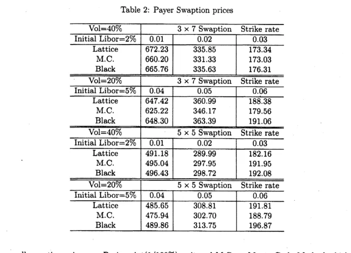
numerical exampleWe calculate the payer swaption of3 $\cross 7$ and 5 $\cross 5$
cases
offlat Libor and volatilities strucure,where Libor are (i) 2% (ii) 5% and the volatilities
are
$(a)0.4(b)0.2$.
These maturities are $3\cross 7$swaption for strike swap-rates for case of (i) are 1%, 2% and 3%. For the case of (ii) strike
swap-rates are 4%, 5% and 6%. We compare the binomial lattice, Monte Carlo method and
Black formula which assumption is Swap market model.
Table 2: Payer Swaption prices
all swaption prices
are
Basis
point(1/100%) unit andM.C.are Monte Carlo
Method whichare
provided by Dr. Yasuoka, MizuhoInformation&Reseach
Insitute, (100,000 runs))Lattice method prices
are
1000
node fora
yearand total stepsare
$1000\cross x$forswaption maturity$x$ years.
From inconsistency of Libor market model and Swap market model, we could have arbtrage
opportunity if we had constructed a hedging strat$e$gy. Davis [2] has shown the existence of
negative libor rate in the
case
ofcoexistense ofLibor and swap market models.For the swaption if
we
take Gaussian model, the hedging strategy isas
follows,$dC(t)=N(d_{n})dB_{n}(t)-N(d_{N})dB_{N}(t)-k \delta\sum_{i=n+1}^{N}N(d_{i})dB_{i}(t)$
which is $e$asily shown. Delta hedging is change of the portfolio which is $N(d_{i})$ unit of bond of
maturity $T_{i}$
.
The hedging strategy ofswap market model is obtained from (5.2)
Provided the longer term interest is changed, the delta hedging of swap market model is not
senstive due to the
same
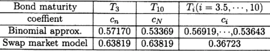
delta $N(d_{2})$ for all$dB_{l}(t)$. The price differencesare caused bycoeffients$c_{i}$
as
Table 1. We calculate coefficient for 3x7swaption (volatity=40%,interest=2%,
strike=2%).
Table 3: Payer swaption $co$effients
In this data case,
we
can see
in Table 3 the $B_{n}(t)$ trading amount is excessive and othermaturity bonds trading is insufficient inswapmarketmodel. Forthis
case we
could take arbitrageopportunityif change of longer term interest shiftupwardand
we
trad$e$swaption and the hedgingstrategy of bonds.
References
[1] Brigo, D Interest Rate Models Theory and Practice, Springer
2001
[2] Davis, M.H.A., and Mataix-Pastor, V. Negative Libor Rates in the Swap Market Model.
Finance and Stochastics 11(2), pp 181-193, (2007)
[3] Jamshidian, F. Libor and SwapMarket Models and Measures, Sakura Global Capital,
1996
[4] Jamshidian, F. Bivariatesupport offorwardLibor andswap rates. Univ. of Twente working
paper, (2005)