RECTIFIABLE, UNRECTIFIABLE AND FRACTAL OSCILLATIONS OF SOLUTIONS OF LINEAR AND HALF-LINEAR DIFFERENTIAL EQUATIONS OF SECOND-ORDER (New Developments of Functional Equations in Mathematical Analysis)

RECTIFIABLE, UNRECTIFIABLE AND FRACTAL OSCILLATIONS OF SOLUTIONS OF LINEAR AND HALF-LINEAR

DIFFERENTIAL EQUATIONS OF SECONKORDER

MERVANPASIC

Abstract. Inthisexpository paper,we payattentiontoa newkind ofoscillations of solutions of

thesecond-orderdifferential equationsonthe finite interval. Itis the so-calledrectifiable,

unrec-tifiable andfractal oscillations ofreal functions and solutions ofdifferential equations introduced

inPaSi\v{c}[S], [9]andWong[15],andcontinuedto studyin[4], [6], [10],[11], [12],and[16].

1. Motivationfortheoscillations

near

$x=0$

Weconsider famous Euler lineardifferentialequation,

$y”+\lambda x^{-2}y=0,$ $x\in(0,\infty),$ $\lambda>0$

.

(1)

DEFINITION 1. A function$y(x)$ oscillates

near

$x=0$ ifthere is

a

decreasing

se-quence

$a_{n}\in(0,1]$ such that $a_{n}\searrow 0$ and $y(a_{n})=0$

.

A fimction$y(x)$ oscillates

near

$x=\infty$ifthere is

an

increasing

sequence

$a_{n}\in[T,\infty)$,for

some

$T>0$,such that $a_{n}arrow\infty$

.

The following basicfacts

on

the equation (1)

are

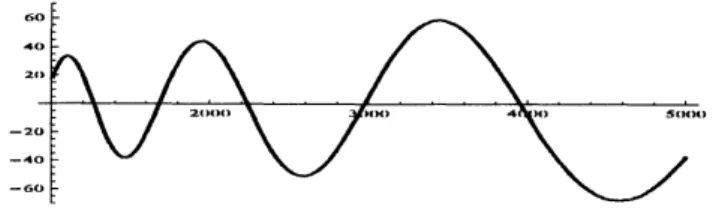
verywellknown:

$\bullet$ if$\lambda>1/4$,thenall solutions$y(x)$ of (1)

are

givenbythe formula

$y(x)=c_{1}\sqrt{x}\cos(p\ln x)+c_{2}\sqrt{x}\sin(\rho\ln x)$,

where $\rho=\sqrt{\lambda-1}/4$;

$\bullet$ $y(x)$

are

oscillating

near

both$x=0$ and$x=\infty$,

see

Figures 1 and2below:

Figure 1: oscillations

near

$x=0$

Mathematics subject_{classification}(2000): $26A27,26A45,28A75,28A80,34B05,34C10,34C20$.

Keywords andphrases: oscillations, linear and half-linear equations, singular, Dirichlet boundary

value problem, graph,rectifiability, $\hslash actal$dimension,Minkowskicontent,asymptotics.

Figure2: oscillations

near

$x=\infty$

2. Definition oftherectiflable and unrectifiableoscillations

on

$[0,1]$

Let $G(y)\subseteq \mathbb{R}^{2}$ denotethegraphof

a

mnction_{$y:[0,1]arrow \mathbb{R}$},defined by $G(y)=\{(x,y)\in \mathbb{R}^{2} : x\in[0,1],y=y(x)\}$

.

Itslengthisdefined by:

length$G(y)= \sup\sum_{i=1}^{m}||(t_{i},y(t_{i})-(t_{i-1},y(t_{i-1}))||_{2}$,

where $0=t_{0}<t_{1}<\cdots<t_{m}=1$ is

a

partitionoftheunitinterval. Ofcourse,in the

case

when$y\in C^{1}((0,1])$,then the length of$G(y)$

can

becalculatedby the formula,

length$G(y)= \lim_{\deltaarrow 0}\int_{\delta}^{1}\sqrt{1+y^{\prime 2}(x)}dx$

.

DEFINITION 2. A Rmction$y(x)$ is

rectifiable

oscillatory

on

$[0,1]$ if$y(x)$

oscil-lates

near

$x=0$ and length$G(y)<\infty$

.

A $fi\iota nctiony(x)$ is

unrectifiable

oscillatory

on

$[0,1]$ if$y(x)$ oscillates

near

$x=0$ and length$G(y)=\infty$

.

EXAMPLE 1. Allsolutions ofthe Euler equation

$y”+\lambda x^{-2}y=0,$_{$x\in(0,1],$ $\lambda>1/4$},

are

rectifiable oscillatory

on

$[0,1]$,where$y(x)$

are

explicitlygivenby:

$y(x)=c_{1}\sqrt{x}\cos(\rho\ln x)+c_{2}\sqrt{x}\sin(p\ln x),$ $\rho=\sqrt{\lambda-1}/4$

.

EXAMPLE 2. All solutions $y(x)$ ofthe linearequation, $y”+\lambda x^{-4}y=0,$$x\in(0,1],$ $\lambda>0$,

areunrectffiable oscillatoryon $[0,1]$,where$y(x)$

are

explicitlygivenby:

3. Rectifiableand unrectiflable oscillations of linear differential equations Accordingto Examples 1 and 2, it is namraly to pose the following questions: what is about the rectffiable and unrectffiable oscillations of the linear second-order differentialequationof Eulertype:

$y”+\lambda x^{-\sigma}y=0,$ $x\in(0,1]$, (2)

where $\lambda>0$ and $\sigma\geq 2$? Does it depend

on

thevaluesof $\sigma$? Inparticular for $\sigma=2$

and $\sigma=4$,the

answer

is given inExamples 1 and 2. However,

a

complete

answer

to

thisquestion is

given

in thefollowingresult. THEOREM 1. We have:

(i)

_if

$2\leq\sigma<4$, thenallsolution

of

Eq.(2)

are

rectifiable

oscillatory

on

$[0,1]$;

(ii)

_if

$\sigma\geq 4$, thenall solution

of

Eq. (2)

are

unrectifiable

oscillatoryon $[0,1]$

.

The proof of Theorem 1

was

published in [8] and [15]. Precisely, Theorem 1 in [8]

was

considered where the followingproperties ofsolutions$y(x)$ of Eq.(2)

are

presumed:

$|y(x)|\leq cx^{\sigma/4}$ and $|y^{f}(x)|\leq cx^{-\sigma/4}$

near

_$x=0$

.

In [15],the previous statementis verified for all solutions of the equationEq.(2),

see

alsoLemma4 below.

The proofof Theorem 1 is based

on

the followingtwolemmas.

LEMMA 1. (see [8])Let$y\in C([0,1])$ oscillate

near

$x=0$. Let $s_{n}\in(0,1]$ bea

decreasingsequence, $s_{n^{\backslash }\searrow}0$ and$y^{f}(s_{n})=0$

.

Thenwe have:

length$G(y)<\infty$

if

and only

if

$\sum_{n=1}^{\infty}|y(s_{n})|<\infty$

.

LEMMA 2. Let $y(x)$ be a solution

of

Eq. (2). Let $s_{n}\in(0,1]$ be a decreasing

sequence, $s_{n}\searrow 0$ and$y’(s_{n})=0$

.

Then thereare twopositive constants $c_{1}$ and $c_{2}$

suchthat:

(i)(see [15])

$c_{1}s_{n}^{\sigma/4}\leq|y(s_{n})|\leq c_{2}s_{n}^{\sigma/4}(i. e. |y(s_{n})|\sim s_{n}^{\sigma/4})$,

(ii) (see [8])

$c_{1}n^{-2/(\sigma-2)}\leq s_{n}\leq c_{2}n^{-2/(\sigma-2)}(i. e. s_{n}\sim n^{-2/(\sigma-2)})$

.

Involving the preciseasymptotic behaviourof$s_{n}$ and $|y(s_{n})|$ from Lemma2 intoLemma

1,

we

getthe proof of Theorem 1.

The result of Theorem 1 could be generalizedto the general linear differential equations:

where $f\in C^{2}((0,1])$ satisfies:

$f(x)>0$ and$f’(x)<0$

on

$(0,1],$ $f(O+)=\infty$, ₍₄₎

$\sqrt{f}\not\in L^{1}(0,1)$ and $f^{-1/4}(f^{-\iota/4})’’\in L^{1}(0,1)$

.

₍₅₎

THEOREM2. Let $f(x)$

satisff

the conditions (4) and (5). Then all solutions

of

Eq. (3) oscillate

near

$x=0$

.

Moreover

length$G(y)<\infty\iota f$and only

if

$\int_{0+}^{1}\sqrt[4]{f(x)}dx<\infty$

.

Theproofof Theorem 2

was

publishedin [4]. It is basedon the following three lemmas.

LEMMA 3. (seethe book[1])Let$y\in C([0,1])$. Then

we

have:

length$G(y)<\infty$

if

andon$ly$

if

$\int_{0+}^{1}|/(x)|dx<\infty$.

LEMMA4. (see [15])Let $f(x)$

satisff

(4) and (5). There_is

a

_{positive constant}

$c$ such that

for

all solutions ofEq. (3) wehave:

$|y(x)| \leq\frac{c}{\sqrt[4]{f(x)}}$ and $|y’(x)|\leq c\sqrt[4]{f(x)}$nearx$=0$.

LEMMA 5. Let $y(x)$ be a solution

of

Eq.(3). Let $s_{n}\in(0,1]$ be a decreasing

sequence, $s_{n}\searrow 0$ and$y’(s_{n})=0$

.

Thereare _{$c_{1}>0$} and$n_{0}\in \mathbb{N}$ such that

$\frac{c_{1}}{\sqrt[4]{f(s_{n})}}\leq[\gamma(s_{n})|,$ $\forall n\geq n_{0}$ and $\int_{s_{n}}^{1}\sqrt{f(x)}dx\sim n$ as$narrow\infty$

.

It is not difficult to check that the fimction $f(x)=x^{-\sigma},$ $x\in(0,1]$ and $\sigma>2$,

satisfiestheconditions (4) and (5). Moreover,

$\int_{0+}^{1}\sqrt[4]{f(x)}dx<\infty$ ifand only if $\sigma<4$

.

Hence, Theorem 1 is

an

easy

consequence

ofTheorem2. 4. Someconsequencesof Theorem2

Accordin$g$to Theorem2,

we are

ableto establishthe rectffiable andunrectifiable

oscillations for

some

classes of linear differential equations which

are

different than the Euler type Eq.(2).

COROLLARY 1. Let $f(x)$

satisff

the conditions (4) and (5). Let $f(x)\sim x^{-\sigma}$

near

$x=0$

.

Then

we

have:

(i)

if

$2\leq\sigma<4$_, then all solution$ofy”+f(x)y=0,$ $x\in(0,1]$,

are

rectifiable

oscillatory

on

the interval $[0,1]$;

(ii)

if

$\sigma\geq 4$, thenall solution

of

$y”+f(x)y=0,$ $x\in(0,1]$,

are

unrectifiable

oscillatory

ontheinterval $[0,1]$

.

COROLLARY2. Weconsider thefollowing chirp’sequation

$y”+x^{-2}[\beta^{2}x^{-2\beta}+(1-\beta^{2})/4]y=0,$$x\in(0,1]$

.

(6)

Thenwehave:

(i)

if

$0<\beta<1$, thenall solution ofEq.(6)

are

rectifiable

oscillatory

on

$[0,1]$;

(ii)

_if

$\beta\geq 1$, then all solution

of

Eq. (6) are

unrectifiable

oscillatoryon $[0,1]$.

COROLLARY 3. (seeWong[15]) Weconsiderthefollowing linear equation

$y”+\lambda x^{-4}e^{\frac{2}{X}}y=0,$ _$x\in(0,1],$ $\lambda>0$

.

(7)

Then all solutionofEq. (7)

are

_{unrectifiable}

oscillatory

on

$[0,1]$

.

5. OnHartman-Wintnerconditions

Let

us

recall that theHamnan-Winmerconditions (5) playstheesential roleinthe proof of Theorem 2. Therefore,it is worthiletofindthe

answer

to the followingopen question: does it possibleto construct thecoefficient $f(x)$ satisfying (4) andthe first

Hartman-Wintner condition ffom (5) but does not satisfy the second

one

ffom (5)? Thatistosay,

we

would liketofind$f(x)$ with the followingproperties:

$f(x)>0$ and $f’(x)<0$

on

$(0,1],$ $f(O+)=\infty$, (8)

$\sqrt{f}\not\in L^{1}(0,1)$ and $f^{-1/4}(f^{-1/4})’’\not\in L^{1}(0,1)$

.

(9)

Inthe solving ofthis problem,wefind that the following lemma could be ofsome interest.

LEMMA 6. Let $f(x)$

satisff

(8) and the second Hartman-Vflntnercondition

from

(5). Then $f(x)$ must

satisfi

the

first

Hartman-Wmtner condition

fivm

(9) and the

followingtwo:

$\lim_{xarrow 0}\Gamma^{3}2(x)f(x)=0$ and $[\Gamma^{3}2f]’\in L^{1}(0,1)$

.

In orderto

prove

this lemma,

we

suggest readerto follow

a

methodpresentedinthe proof of[11,Lemma2].

6. Coexistenceof the rectiflableand unrectifiable oscillations AccordingtoTheorem2,weobserve the followingconsequence.

COROLLARY4. Let$f(x)$ satisfythecondition (4) and (5). _Let$y_{1}(x)$ and$y_{2}(x)$

be two linearly independentsolutions

_of

$y”+f(x)y=0,$ $x\in(0,1]$. Then $y_{1}(x)$ and $y_{2}(x)$

are

both

rectifiable

oscillatory

on

_$[0,1]$ atthe

same

time.

Hence it is reasonable topose the following question: it is possible to constmct the coefficient$f(x)$ satisfying (8) and (9) such that$y_{1}(x)$ isrectffiable andatthe

same

time$y_{2}(x)$ is unrectffiable oscillatoryonthe interval _$[0,1]$?

The

answer

is yes andit could be found in the last section of[4].

7. Rectifiableand unrectifiable oscillations of solutions of the half-linear differential equations

Inthissection,

we

consider half-linear differential equation,

$(|y’|^{p-2}y’)’+f(x)|y|^{p-2}y=0,$ $x\in(0,1]$, (10)

where $f(x)$ besides (4) satisfies the following Hartman-Wintner_{typeconditions}

gen-eralizing the related

ones

in (5) from$p=2$ to $p>1$:

$f^{\frac{1}{p}}\not\in L^{1}(0,1)$ and $f^{-\frac{1}{pq}}[f^{-2^{1}}p]’’\in L^{1}(0,1)$

.

(11)

Inparticularfor$p=2$,obviouslyEq. (10) becames the linear equationEq. (3) consid-ered in previoussections. The following resultis

a

naturalgeneralization of Theorem2 from lineartothehalf-linearequations.

THEOREM 3. Let$f(x)>0$and$f’(x)<0$

on

$(0,1],$ $f(O+)=\infty$ andsatisfy (11).

Then all solutions ofEq.(10) oscillatenear$x=0$_. Moreover,

length$G(y)<\infty\iota f$andonly$\iota f\int_{0+}^{1}f^{\frac{1}{p^{2}}}(x)dx<’\infty$

.

The proofofTheorem 3 has been publishedin [11]. It is based

on

the follwing two steps.

Firststep. Every solution$y(x)$ ofEq.(10) could bewrittenin the form:

$y(x)=(p-1)^{\frac{1}{pq}}\Gamma^{\frac{1}{pq}}(x)\nabla^{\frac{1}{p}}(x)w(\varphi(x))$,

$|/|^{p-2}y’=-(p-1)^{-\frac{1}{pq}}f^{\frac{1}{pq}}(x)\nabla^{\frac{1}{q}}(x)|w’(\varphi(x))|^{p-2}w^{f}(\varphi(x))$,

where the fimction $w=w(t),$ $t>0$, istheso-calledgeneralizedsinehnction,

$|\sqrt{}(t)|^{p}+|w(t)|^{p}\equiv 1$ for all $t>0$

.

Secondstep. Itis importantto showthat the ffinctions $V(x)$ and $\varphi(x)$

satis

$\theta$the

equations:

$\varphi’(x)=\frac{-1}{(p-1)^{\frac{1}{p}}}f^{\frac{1}{p}}(x)+\frac{1}{p}\frac{f(x)}{f(x)}|\sqrt{}(\varphi(x))|^{p-2}w’(\varphi(x))w(\varphi(x))$ ,

$V’(x)=[(p-1)^{\frac{1}{p}}\Gamma^{\frac{1}{p}}(x)]’|y’|^{p}+[(p-1)^{-\frac{1}{q}}f^{\frac{1}{q}}(x)]’|y|^{p}$,

andthe following

asymptotic

conditions:

$\varphi’(x)<0$ for all $x\in(0,1]$ and $\lim_{xarrow 0+}\varphi(x)=\infty$, $0< \lim_{xarrow 0+}\nabla(x)<+\infty$

.

Now,accordingtotheprevioustwo stepsandby using the

same

geometric

lemmas

as

in the of Theorem2,

one can

derive the proof of Theorem3.

8.

Furthergeneralization: two-point oscillations

Inthissection,

we

presentthe oscillationsofsolutionsofthe$D\ddot{m}chlet$problem

on

theunitinterval which

was

introducedin[12].

DEFINITION 3. Afimction$y(x)$ istwo-point oscillatory

on

$[0,1]$ if$y(x)$ oscillates

at the

same

time

near

$x=0$ and $x=1$

.

That is, if there is

a

decreasing

sequence

$a_{n}\in$ $(0,1]$ andincreasing

sequence

$b_{n}\in[0,1)$ such that: $a_{n}\searrow 0,$ $b_{n}\nearrow 1$,and$y(a_{n})=$

$y(b_{n})=0$,

see

figure below:

Figure 3: two-point oscillationswith higher density

near

$x=0$ and$x=1$

Themain

motivation

to study this kind ofoscillations

we

obtainffomthe oscilla-tions oftheso-called Riemann-Weber versionof Euler lineardifferentialequation,

$y”+x^{-2}( \frac{1}{4}+\frac{\lambda}{|\ln x|^{2}})y=0,$$x\in(0,1),$ $\lambda>0$

.

(12)

$\bullet$ if$\lambda>1/4$,then all solutions$y(x)$ of(12)

are

given by the fonnula: $y(x)=\sqrt{x\ln\frac{1}{x}}[c_{1}\cos$

(

$p$ln ln$\frac{1}{x}$

)

$+c_{2}\sin$

(

$p$ln ln$\frac{1}{x}$

)

$]$, where $p=\sqrt{\lambda-1}/4$;

$\bullet$ $y(x)$

are

oscillating

near

$x=0$ and $x=1$ atthe

same

time. 9. Theexistenceoftwo-point oscillations

We startwithtwolinearly independent fimctions$y_{1}(x)$ and$y_{2}(x)$ in the form:

$y1(x)=|q’(x)|^{-}2\cos q(x)1$ _and $y_{2}(x)=|q’(x)|^{-z}\sin q(x)l$

.

It isnot difficult to

see

thatthe equation which corresponds to the hndamentalset of solutions$y(x)=c_{1}y_{1}(x)+c_{2}y_{2}(x)$, it is:

$y”+[ \frac{1}{2}S(q’)(x)+(q’)^{2}(x)]y=0,$ $x\in(O, 1)$, (13)

where $S(q’)(x)$ denotes

as

usualthe Schwarzian_derivativeof$q(x)$ defined by

$S(q’)(x)= \frac{q’’’(x)}{q’(x)}-\frac{3}{2}[\frac{q’’(x)}{q’(x)}]^{2},$ _$x\in(0,1)$.

THEOREM4. Let $q(x)$

satisff

thefollowing condition:

$q\in C^{3}(0,1)$, ₍₁₄₎

$|q(0+)|=|q(1-)|=+\infty$ and $|q^{f}(0+)|=|q^{f}(1-)|=+\infty$, (15)

$q’(x)<0$

_for

all$x\in(O, 1)$ and $S(q’)\in C(O, 1)$

.

₍₁₆₎

Then all solutions

_of

Eq. (13)

are

two-pointoscillatory on $(0,1)$

.

Moreover,

for

any

function

$f\in C(O, 1)$ suchthat

$f(x) \geq[\frac{1}{2}S(q’)(x)+(q’)^{2}(x)],$ _{$x\in(O, 1)$},

then allsolutions

_of

the equation $y”+f(x)y=0,$ $x\in(0,1)$,

are

_two-pointoscillatory

on $[0,1]$.

Theproofofthis theorem hasbeen publishedin [12].

Some classes ofthe frequences $q(x)$ whichsatis$\theta(14),$ (15),and (16)

are

given

alogarithmic class:$q(x)=\rho$lnln$\frac{1}{X},$$\rho=\sqrt{\lambda-\frac{1}{4}}$ apolynomial class:$q(x)= \frac{1-2r}{(x-x^{2})^{\beta}},$$\beta>0$

10. Some

consequences

ofTheorem 4

COROLLARY 5. Let $\rho=\sqrt{\lambda-\frac{1}{4}}$ and $\lambda>\frac{1}{4}$

.

Then all solutions

of

Riemann-Weberequation (13)

are

two-pointoscillatoryon $[0,1]$.

Proof.

The fimction$q(x)=p$lnln$\frac{1}{X}$ satisfies the conditions (14), (15), and (16).

Moreover,

$\frac{1}{2}S(q’)(x)+(q^{f})^{2}(x)=x\urcorner 1(\frac{1}{4}+\frac{\lambda}{|\ln x|^{2}})$ ,

and thus:

$y”+ \frac{1}{x^{2}}(\frac{1}{4}+\frac{\lambda}{|\ln x|^{2}})y=y’’+[\frac{1}{2}S(q’)(x)+(q’)^{2}(x)]y=0,$ $x\in(0,1)$

.

Hence by Theorem 4, all solutions of

Riemann-Weber

equation (13)

are

two-point oscillatory

on

$[0,1]$

.

Q.E. D.

COROLLARY 6. Let $c(x)$ besmooth andpositive

on

$[0,1]$ and let $\sigma>2$. Then

all solutions

_of

theequation;

$y”+ \frac{c(x)}{(x-x^{2})^{\sigma}}y=0,$$x\in(0,1)$, (17)

aretwo-point$oscillato,y$on $[0,1]$

.

Proof

At the first, the ffinction $q(x)= \frac{1-2\mathfrak{r}}{(x-x^{2})^{\beta}},$ $\beta>0$, satisfies the conditions

that $2\beta+2<\sigma$ and

$f(x):= \frac{c(x)}{(x-x^{2})^{\sigma}}\geq\frac{m}{(x-x^{2})^{2\beta+2}}\geq[\frac{1}{2}S(q’)(x)+(q’)^{2}(x)]$,

where $q(x)= \frac{1-2\mathfrak{r}}{(x-x^{2})^{\beta}}$. Hence by Theorem 4, all solutions of Eq.(17)

are

two-point

oscillatory

on

$[0,1]$

.

Q.E. D.

COROLLARY 7. Let $c(x)$ be a

continuousfunction

on $[0,1]$ such that $c(x)\geq 1$

for

all$x\in(0,1)$. Then all solutions

of

the_equation:

$y”(x)+c(x)e^{\frac{4}{x-x^{2}}}y(x)=0,$ _{$x\in(O, 1)$, (18)}

are

two-pointoscillatory

on

$[0,1]$.

Proof.

Thefimction $q(x)=(1-2x)e^{\frac{1}{x-x^{2}}}$ _{satisfies the conditions}

(14), (15), and (16). Now,

we

have:

$f(x):=c(x)e^{\frac{4}{x-x^{2}}} \geq\frac{e^{\chi-X}=^{2}}{(x-x^{2})^{4}}\geq[\frac{1}{2}S(q’)(x)+(q’)^{2}(x)]$

,

where $q(x)=(1-2x)e^{\frac{1}{x-x^{2}}}$

.

_{Hence byTheorem}

4, all solutions of Eq. (18) are

two-point oscillatory

on

$[0,1]$

.

Q. E.D.

11. Two-point rectifiableand unrectifiable oscillations

DEFINITION 4. A Rmction $y(x)$ is two-point

rectifiable

oscillatory

on

$[0,1]$ if $y(x)$ is two-point oscillatoiy on $[0,1]$ and length$G(y)<\infty$. A hnction $y(x)$ is

two-point

_{unrectifiable}

_oscillatory

_on

$[0,1]$ if$y(x)$ is two-point oscillatory

on

$[0,1]$ and

length$G(y)=\infty$.

THEOREM 5. Let $q(x)$

satisff

the previous conditions (14), (15), and (16).

There holds true:

(i)$\iota f(|q’|^{-2}3|q’’|+|q’|^{1}z)\in L^{1}(0,1)$_, then all solutions ofEq.₍₁₃₎

_are

_two-point

rectifi-ableoscillatory on $(0,1),\cdot$

(ii) $\iota f|q’(x)|^{-1}$ isincreasing

near

_$x=0$ anddecreasing

near

_$x=1$ andthe_series, $\sum_{k}|q’(q^{-1^{1}}(k\pi))|^{-z}$ $or$ $\sum_{k}|q’(q^{-1}(-k\pi))|^{-z^{1}}$

is divergent, then allsolutions

_of

Eq.(13) are two-point

_{unrectifiable}

$oscillato,y$ on

$(0,1)$.

COROLLARY 8. Let $c(x)$ besmooth andpositive

on

$[0,1]$

.

Wehave:

(i)

_if

$\sigma\in(2,4)$_, then equation (17) is two-point

rectifiable

oscillatory

on

$[0,1]$

.

(ii)

_if

$\sigma\geq 4$, then equation (17) is two-point

unrectifiable

oscillatoryon $[0,1]$

.

Theproofs ofTheorem5 and Corollary8have been publishedin[12].

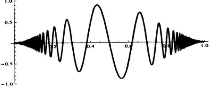
12. Motivation tointroduce and study theso-called fractal oscillations Inthe application (acoustic, telecomunication, signal processingetc.),

a

signal is called chirpifits ffequence isgrowing up

or

down in the time:

Figure4: the $(\alpha,\beta)$-chirp: $y(x)=x^{\alpha}\cos(x^{-\beta})$

or

$y(x)=x^{\alpha}\sin(x^{-\beta})$

On the rectffiable andunrectffiableoscillationsofthe $(\alpha,\beta)$-chirp

one can

saythe

following.

THEOREM 6. (see the book [14]) Let $y(x)$ be the $(\alpha,\beta)$-chirp, that is, $y(x)=$ $x^{\alpha}\cos(x^{-\beta})$ or$y(x)=x^{\alpha}\sin(x^{-\beta})$

.

Then wehave:

lengthG$(y)=\infty$ $\Leftrightarrow$ $\beta\geq\alpha$

.

How to estimate the density of

an area

filled by

a

chirp

near

$x=0$,

see

figure above? In ordertogivethe

answer

tothisquestion,

we

needtorecall

some

notionsffom the ffactalgeometryof plane

curves

like the $\epsilon$-neighbourhood, Minkowski-Bouligand

dimension (box dimension) and the s-dimensional Minkowski content of the graph

$G(y)$ denotedrespectively by $G_{\epsilon}(y),$ $\dim_{M}G(y)$ and $M^{s}(G(y))$, and defined

respec-tivelyby:

$G_{\epsilon}(y)=\{(t_{1},t_{2})\in \mathbb{R}^{2} : d((t_{1},t_{2}),G(y))\leq\epsilon\}$,

$\dim_{M}G(y)=\lim_{\epsilonarrow 0}(2-\frac{\log|G_{\epsilon}(\gamma)|}{\log\epsilon})$ ,

$W(G(y))= \lim_{\epsilonarrow 0}(2\epsilon)^{s-2}|G_{\epsilon}(y)|,$ $s\in[1,2]$

.

Let

us

remark that in the general case, in previous definitions it is required the tenn

Itis$elemental\gamma$toobtain the following properties:

(i) $|G_{\epsilon}(y)|arrow 0$

as

$\epsilonarrow 0$ and the densityofan

area

filled by _$G(y)$ isequivalent

tothe asymptotics of $|G_{\epsilon}(y)|$

as

$\epsilonarrow 0$;

(ii) $\dim_{M}G(y)=s,$ $0<M^{s}(G(J))<\infty$ $\Leftrightarrow|G_{\epsilon}(y)|\sim\epsilon^{2-s}$

as

$\epsilonarrow 0$

.

Now, the density of

an

area

filledby

a

chirp

near

$x=0$, _{it could be described by}

thefollowingresult.

THEOREM 7. (see the book [14]) Let$y(x)$ be the $(\alpha,\beta)$-chirp, that is, $y(x)=$ $x^{\alpha}\cos(x^{-\beta})$ or$y(x)=x^{\alpha}\sin(x^{-\beta})$

.

Thenwehave:

$\dim_{M}G(y)=2-\frac{1+\alpha}{1+\beta}$ and $|G_{\epsilon}(y)|\sim\epsilon^{\frac{1+\alpha}{1+\beta}}$

as $\epsilonarrow 0$

.

Let

us

remarkthat the box dimension satisfies the followingaxiomatic properties. Thatis, if$P(\mathbb{R}^{2})$ denotesthepartitivesetof$\mathbb{R}^{2}$,thenwe

have:

(i) $\dim_{M}:P(\mathbb{R}^{2})arrow[1,2]$;

(ii) if$E\subseteq F$,then _{$\dim_{M}(E)\leq\dim_{M}(F)$} (monotonicity);

(iii) $\dim_{M}(E\cup F)=\max\{\dim_{M}(E),\dim_{M}(F)\}$ (finite stability);

(iv)if$f$: $\mathbb{R}^{2}arrow \mathbb{R}^{2}$ is

a

bi-Lipschitztransformation,then for all $E\subseteq \mathbb{R}^{2}$,

$\dim_{M}(f(E))=\dim_{M}(E)$ (bi-Lipschitzinvariance).

13. Fractaloscillationsof realfunctions

Now,

we

recall the definitionofthe so-called fractal oscillations of realhnctions introducedin[9].

DEFINITION 5. Let $s\in[1,2]$

.

A hnction$y(x)$ is the _{$s-dimensionalfi^{d}actal$}

oscil-latory

on

$[0,1]$ if$y(x)$ oscillates

near

$x=0$ and$\dim_{M}G(y)=s$ and$0<W(G(y))<\infty$

.

A fUnction$y(x)$ is called tobe

fractal

oscillatory

on

$[0,1]$ ifthereis

an

$s\in[1,2]$ such

that$y(x)$ isthe

s-dimensionalfractal

oscillatory

on

$[0,1]$

.

THEOREM 8. (ageneralizationofTheorem7)Let$y(x)$ be the $(\alpha,\beta)$-chirp, that

is, $y(x)=x^{\alpha}\cos(x^{-\beta})$ or$y(x)=x^{\alpha}\sin(x^{-\beta})$

.

Thenwehave:

(i)

_if

$\alpha>\beta>0$_, then$y(x)$ isthe l-dimensional

fractal

oscillatoryon $[0,1],\cdot$

(ii)

_if

$\alpha=\beta>0$, then $y(x)$ isnot

fractal

oscillatory on $[0,1]$, since $\dim_{M}G(y)=1$

and$M^{1}(G(y))=\infty$;

(iii) $lf0<\alpha<\beta$, then $y(x)$ is the s-dimensional

fractal

oscillatoryon $[0,1]$, where

14. Fractaloscillations of lineardifferential equations

Suchakind ofresults presented in Theorem8,it could be also verifiedtothe

case

of all solutions of linear differentialequationsofsecond-order.

DEFINITION 6. Let $s\in[1,2]$ be

an

arbitrarilygivenrealnumber. Alinear

equa-tion $(P):y”+f(x)y=0$ is saidtobethe s-dimensional ffactal oscillatory

on

$[0,1]$,if

allits solutions$y(x)$

are

the

s-dimensionalfractal

oscillatory

on

$[0,1]$

.

Weknow that:

$\bullet$ Euler equation

$y”+\lambda x^{-2}y=0,$ $x\in(0,1],$ $\lambda>1/4$,

isthe

_{l-dimensionalffactal}

oscillato$y$

on

$[0,1]$;

$\bullet$ The (2, 3)-chirpequation,

$y”+(9x^{-8}-2x^{-2})y=0,$ $x\in(O, 1]$,

isthe s-dimensional ffactal oscillatory

on

$[0,1]$,where $s=5/4$

.

What isabout the ffactal oscillations of the linear second-order differential equa-tion of Eulertype:

$y”+\lambda x^{-\sigma}y=0,$ _{$x\in(O, 1]$}, (19)

where $\lambda>0$ and $\sigma\geq 2$? Does

it

depend

on

the values of$\sigma$? The

answer

is

given

in

the following result.

THEOREM 9. Wehave:

(i)$\iota f2\leq\sigma<4$, then Eq.(19) isthe

l-dimensionalfractal

oscillatory

on

$[0,1],\cdot$

(ii)

_if

$\sigma=4$_, then Eq.(19) is

notfractal

oscillatory

on

$[0,1]$_,since$\dim_{M}G(\gamma)=1$ and $M^{1}(G(y))=\infty$;

(iii)

_if

$\sigma>4$_, thenEq. (19) isthe

s-dimensionalfiactal

oscillatoryon _$[0,1]$, wherethe

dimensional number$s$

satisfies

$s= \frac{3}{2}-\frac{2}{\sigma}$

.

REMARK 1. For $\sigma=4$

we

have

a

kindofthe s-dimensionalMinkowski

degener-ation. That is,theequation,$y”+\lambda x^{-4}y=0,$_$x\in(0,1],$ $\lambda>0$, isnotffactal oscillatory

on $[0,1]$,since $\dim_{M}G(y)=1$ and$M^{1}(G(y))=\infty$ for all solutions$y(x)$

.

That is, $G(y)$

isnot $M^{1}$ measurable.

The proof ofTheorem9has been published in [9].

Next,

we

consider the linear second-order differentialequation:

$y”+f(x)y=0,$ $x\in(0,1]$, (20)

where $f\in C^{2}((0,1])$ satisfies:

$f(x)>0$ and$f^{f}(x)<0$

on

$(0,1],$ $f(O+)=\infty$, (21)

THEOREM 10. Let$f(x)sa\hslash sff$the conditions (21) and(22), andlet_{$f(x)\sim x^{-\sigma}$}

near$x=0$

.

_Thenwehave:

(i)$\iota f2\leq\sigma<4$_, thenEq. (20) is the

l-dimensionalfractal

oscillatoryon _{$[0,1],\cdot$}

(ii)$lf\sigma=4$, then Eq.(20) is

notffactal

_oscillatoryon_{the interval}$[0,1]$_,since$\dim_{M}G(y)=$

$1$ and $M^{1}(G(y))=\infty$;

(iii)$\iota f\sigma>4$_, then Eq. (20) isthe

s-dimensionalfractal

oscillatoryon _$[0,1]$

, where the

dimensional number$s$

satisfies

$s= \frac{3}{2}-\frac{2}{\sigma}$.

TheproofofTheorem 10has beenpublishedin [4].

Asa

consequence

weobserveageneralization ofTheorem 8. COROLLARY 9. Weconsiderthe $(\alpha,\beta)$-chirpequation:

$y”+( \frac{\beta^{2}}{x^{2\beta+2}}+\frac{1-\beta^{2}}{4x^{2}})y=0,$

$x\in(0,1]$, (23)

where $\alpha=(\beta+1)/2$. Thenwehave:

(i)$\iota f0<\beta<1$_, then Eq.(23) isthe

l-dimensionalfractal

oscillatory

on

_{$[0,1],\cdot$}

(ii)

_if

$\beta=1$_, then Eq. (23) is

notfractal

oscillatory on _{$[0,1]$,since $\dim_{M}G(y)=1$ and}

$M^{1}(G(y))=\infty$;

(iii)$tf\beta>1$, thenEq. (23) isthe

s-dimensionalfractal

_{oscillatoryon} $[0,1]$, wherethe

dimensionalnumber $s$

satisfies

$s= \frac{3}{2}-\frac{1}{\beta+1}$

.

15. Whatis the

essences

in the fractaloscillations? Thefollowingstatements

are

equivalent:

(i)$y(x)$ isfractal oscillatory

on

$[0,1]$;

(ii)there isan$s\in[1,2]$ such that:

$\dim_{M}G(y)=s$ and $0<M^{\theta}(G(J))<\infty$;

(iii) $|G_{\epsilon}(y)|\sim\epsilon^{2-s}$ when $\epsilonarrow 0$,that is, there

are

_{$c_{1},c_{2}>0$} suchthat:

$c_{1}\epsilon^{2-s}\leq|G_{\mathcal{E}}(J)|\leq c_{2}\epsilon^{2-s}$ forsmall $\epsilon>0$

.

Hence, in orderto prove that

an

oscillatory ffinction $y(x)$ is the ffactaloscillatory

on

$[0,1]$_,

we

need_toestimate $|G_{\mathcal{E}}(y)|$ from belowandabove by the term $\epsilon^{2-s}$, for

some

$s\in[1,2]$

.

Therefore

one can

observe that the essential tools_{in the ffactal oscillations}

playthefollowingtwolemmas.

LEMMA 7. (a lower bound of $|G_{\mathcal{E}}(y)|$)Let$y\in C([0,1])$ and let _{$a_{n}\in(0,1]$} bea

decreasingsequence

_of

consecutive

zeros

_of

$y(x)$ such that $a_{n}\searrow 0$. Then there is a

function

$k:(0,\epsilon_{0})arrow N$

for

some $q>0,$ $k=k(\epsilon)$_, such that:

$k(\epsilon)$ is increasingand$k(\epsilon)arrow\infty$

as

$\epsilonarrow 0$

.

Moreover,

_for

anyfunction $k(\epsilon)$ satisffing (24) and (25),

we

have

(25)

$\sum_{n=k(\epsilon)^{X}}^{\infty}\max_{\in[a_{n+1}a_{n}]},|y(x)|(a_{n}-a_{n+1})\leq|G_{\epsilon}(y)|$

for

small

$\epsilon>0$

.

(26)

The proof ofLemma7

was

published in[4, Appendix]andin

a

corresponding integral form

in

[7,

Section

2].

REMARK 2. Obviously,the term $\max_{x\in[a_{n+1},a_{n}]}|y(x)|$ in (26) could be replaced

byweaker

one:

$[\gamma(s_{n})|$,where $s_{n}\in[a_{n+1},a_{n}]$

.

LEMMA 8. (an

upper

bound of $|G_{\epsilon}(y)|$)Let $y\in C([0,1])\cap C^{2}((0,1]),$ $y(O)=0$

andlet $a_{n}\in(0,1]$ beadecreasing

sequence

of

inflexion-points

of

$y(x)$ such that$a_{n}\searrow$ $0$. Then thereis

afunction

$m:(0,\epsilon_{0})arrow N$

for

some

$\mathfrak{g}\in(0,1),$ $m=m(\epsilon)$, such that: $|a_{n}-a_{n+1}|\geq 4\epsilon$

for

all$n=1,2,$$\ldots,m(\epsilon)$ and $\epsilon\in(0,\epsilon_{0})$, (27) $m(\epsilon)$ is increasingand$m(\epsilon)arrow\infty$

as

$\epsilonarrow 0$

.

(28)

Next, thereisapositive constant$M>0$ _such

thatfor

anyfunction $m(\epsilon)$ satisfiing (27)

and (28),

we

have

$|G_{\epsilon}(y)| \leq M[\epsilon+a_{m(\epsilon)}\max_{x\in[0,a_{m(\epsilon)}]}|y(x)|]$

$+M[ \epsilon\sum_{n=2^{X}}^{m(\epsilon)}\max_{a_{n}\in[a_{n+1}]},|y(x)|+\epsilon^{2}m(\epsilon)]$

for

small$\epsilon>0$

.

The proof of Lemma 7

was

published in [7, Section 2] in the special

case

when the boundary

curves

of$G_{\epsilon}(y)$

are

regular.

16. Open problem$A$

:

fractal oscillations of self-adjontlineardifferential

equations Inthissection,

we

consider the self-adjont equation:

$(p(x)y’)’+q(x)y=0,$ $x\in(O, 1]$, (29)

where$y\in C([0,1])\cap C^{2}((0,1])$ and the coefficients$p(x)$ and $q(x)$ satis$\theta$

:

$p\in C^{1}([0,1]),$$p(x)>0$ and$p’(x)\geq 0$

on

$(0,1]$, (30)

$q\in C^{2}((0,1]),$ $q(x)>0$ and $q’(x)<0$

on

$(0,1],$ $q(O+)=\infty$, (31)

and satisify thefollowingHartman-Wintnertypeconditions:

$\sqrt{\frac{q}{p}}\not\in L^{1}(0,1)$and $\frac{1}{\sqrt[4]{pq}}(p(\frac{1}{\sqrt[4]{pq}})^{f})’\in L^{1}(0,1)$

.

(32)

CONJECTURE 1. Let the

_functions

$p(x)$ and $q(x)$

satisff

the conditions (30),

(31) and (32), andlet

$p(x)\sim x^{\mu}$ and $q(x)\sim x^{-\sigma}$

near

$x=0$,

where $\mu\geq 0,$ $\sigma>0,$ $\sigma+\mu>2$, and $\sigma-\mu>-4$. Then theequation

$(p(x)y’)’+q(x)y=0,$ $x\in(0,1]$,

is the $s-$

dimensionalfractal

oscillatory on $[0,1]$_, where the dimensional number $s$

satisfies:

$s= \frac{3}{2}+\frac{\mu-2}{\sigma+\mu}$.

It is clear that Conjecture 1 in particular for $p(x)\equiv 1,$ $q(x)=f(x),$ _$\mu=0$, and $\sigma=\sigma$, generalizes both Theorem9 andTheorem 10

on

thefractal oscillations ofthe

equation$y”+f(x)y=0,$ $x\in(0,1]$

.

WhenConjecture 1 isverified,then

we

have the followingconsequence.

COROLLARY 10. (aconditional

consequence

ofConjecture 1)Let$f(x)>0$ and $f(x)<0$ on $(0,1],$ $f(O+)=\infty$ and

satisff

the Hartman-Wintnertypeconditions:

$\sqrt{f}\not\in L^{1}(0,1)$ and $f^{-\iota/4}(f^{-1/4})’’\in L^{1}(0,1)$

.

If

$\mu\geq 0$ and$f(x)\sim x^{-\sigma},$ $\beta\geq 1$, then thelinearequation:

$y”+\mu x^{-1}y^{f}+f(x)y=0,$ $x\in(O, 1]$,

is the s-dimensional

_fractal

oscillatory on $[0,1]$, where thedimensional number $s=$

$\frac{3}{2}+\frac{\mu-2}{\sigma}$.

It isclear that previous conditionalconsequenceof Conjecture 1 inparticular for

$\mu=0$, generalizes both Theorem9 and Theorem 10

on

the fractal oscillations of the

equation$y”+f(x)y=0,$ $x\in(0,1]$

.

Also,itmotivates

a

studypresentedinthefollowing

section.

Some resultsonthe Conjecture 1 willappear in aforthcomingpaper[10].

17. Open problem$B$

:

fractal oscillations of linear differentialequationswith

dampingterm

What kind of asymptotic properties

near

$x=0$

are

proposedto the coefficients

$f(x)$ and$g(x)$ suchthat the linearequation:

$y”+g(x)y’+f(x)y=0,$ $x\in(0,1]$,

isthe s-dimensionalffactal oscillatory

on

$[0,1]$ for

some

$s\in(1,2]$?

A motivation tosolve this problem

we

findinthebook [14],which could be for-mulatedinthisway: if$0<\alpha<\beta$,then the $(\alpha,\beta)$-chirpequation:

.

$y”+ \frac{\beta-2\alpha+1}{x}y’+(\frac{\beta^{2}}{x^{2\beta+2}}-\frac{\alpha(\beta-\alpha)}{x^{2}})y=0,$ _$x\in(0,1]$

.

18. Open problem$C$

:

rectifiable and unrectifiable oscillations ofradially

symmetricsolutions of

some

pde’s

Let$N\geq 2$ and let $B=\{x\in \mathbb{R}^{N}:|x|<1\}$be

a

unit

ballcenteredatthe

origin

with

its boundary $\partial B$

.

DEFINITION 7. A fimction $u:B\backslash \{0\}arrow \mathbb{R}$ is said to be radially symmetric if

thereis

a

Rmction$y=y(r),$$y:(0,1]arrow \mathbb{R}$ such that $u(x)=y(|x|),$ $x\in B\backslash \{0\}$

.

Aradiallysymmetric hnction $u:B\backslash \{0\}arrow \mathbb{R}$ issaidtobe oscillatory

near

$\partial B$ if

cor-respondingfimction$y=y(r)$ _oscillates

near

$r=1$

.

A radially symmetric function $u:B\backslash \{0\}arrow \mathbb{R}$ is said to be s-dimensional

fractal

oscillatory near $\partial B$ if corresponding fimction $y=y(r)$ oscillates

near

$r=1$ and

$\dim_{M}G(y)=s$ and $0<M^{s}(G(y))<\infty$, for

some

$s\in[0,1]$

.

EXAMPLE 3. Weconsiderthe radiallysymmetricsolutionsoftheDirichlet prob-lem:

$\{\begin{array}{l}-\Delta u=\frac{\lambda}{|x|^{2}\ln^{2}|x|}u in B\backslash \{0\}\subseteq \mathbb{R}^{2}, \lambda>1/4,u=0 on\partial B.\end{array}$ (33)

Allradially symmetric solutions $u(x)$ of $(3\dot{3})$

are

the l-dimensional ffactal oscillatory

near

$\partial B$

.

Itisbecause:

$u(x)=\sqrt{\ln\frac{1}{|x|}}[c_{1}\cos(p$ln ln$\frac{1}{|x|})+c_{2}\sin(\rho\ln\ln\frac{1}{|x|})]$ ,

where $x\in B\backslash \{0\}\subseteq \mathbb{R}^{2},\lambda>1/4,$ $\rho=\sqrt{\lambda-1}/4$, and $c_{1},c_{2}\in \mathbb{R}$

.

EXAMPLE4. We considertheradiallysymmetric solutions ofthe$D\ddot{m}chlet$

prob-lem:

$\{\begin{array}{l}-\Delta u=\frac{\lambda}{|x|^{2}\ln^{4}|x|}u in B\backslash \{0\}\subseteq \mathbb{R}^{2}, \lambda>0,u=0 on\partial B,\end{array}$ (34)

Allradially symmetricsolutions $u(x)$ of (34)

are

notffactal oscillatory

near

$\partial B$

.

Itis

because:

$u(x)= \ln|x|[c_{1}\cos(\frac{\sqrt{\lambda}}{\ln|x|})+c_{2}\sin(\frac{\sqrt{\lambda}}{\ln|x|})]$,

where$x\in B\backslash \{0\}\subseteq \mathbb{R}^{2},$ $\lambda>0$ and$c_{1},c_{2}\in \mathbb{R}$

.

Now,

we

consider the one-parameter Dirichlet problem:

$\{\begin{array}{l}-\Delta u=\frac{\lambda}{|x|^{2}(-\ln|x|)^{\sigma}}u in B\backslash \{0\}\subseteq \mathbb{R}^{2}, \sigma\geq 2,u=0 on\partial B,\end{array}$ (35)

CONJECTURE 2. (the

case

when$N=2$) Wehave:

(i)

_if

$2\leq\sigma<4$_, then all radially _{symmetric solutions $u(x)$}

of

_{Eq. (35) are the}

1-$dimensionalf’actal$oscillatorynear $\partial B$;

(ii)

_if

$\sigma=4$_, then radiallysymmetricsolutions _$u(x)$ ofEq.₍₃₅₎ are

notfiactal

oscilla-torynear $\partial B$

, since $\dim_{M}G(y)=1$ and$M^{1}(G(y))=\infty$;

(iii)$lf\sigma>4$, then radiallysymmetricsolutions $u(x)$ ofEq.(35)

are

thes-dimensional

fractal

oscillatorynear $\partial B$, where

the dimensional number$s$

satisfies

$s= \frac{3}{2}-\frac{2}{\sigma}$.

Also,

we

consider theone-parameter$D\ddot{m}chlet$problem:

$\{\begin{array}{l}-\Delta u=\frac{\lambda(2-N)^{2}}{|x|^{2N-2}(|x|^{2-N}-1)^{\sigma}}u in B\backslash \{0\}\subseteq \mathbb{R}^{N},u=0 on\partial B,\end{array}$ (36)

where $u\in C^{2}(B\backslash \{0\})\cap C(\overline{B}\backslash \{0\}),$ _{$N\geq 3,$} $\sigma\geq 2$ and $\lambda>0$

.

CONJECTURE 3. (the

case

when$N\geq 3$) Wehave:

(i) $\iota f2\leq\sigma<4$_, then all radially symmetric solutions $u(x)$

of

Eq.(36) are the

1-dimensionalfractal

oscillatorynear $\partial B$;

(ii)

_if

$\sigma=4$_, then radiallysymmetricsolutions _$u(x)$ ofEq.(36) are

notfactal

oscilla-torynear $\partial B$

,since $\dim_{M}G(y)=1$ and$M^{1}(G(y))=\infty$;

(iii)

_if

$\sigma>4$_, thenradiallysymmetricsolutions _$u(x)$ ofEq. (36) arethe s-dimensional

fractal

oscillatorynear $\partial B$, wherethedimensionalnumber

$s$

satisfies

$s= \frac{3}{2}-\frac{2}{\sigma}$.

For

more

details abouttwoprevious conjecture

we propose

the forthcoming

paper

[6]. REFERENC ES

[1] L. C.EVANSAND R. F.GARIEPY,Measure Theory and Fine Properties_ofFunctions, CRCPress,

NewYork, 1999.

[2] K. FALCONER, Fractal Geometry. Mathematical Fondations and Applications, John Willey-Sons,

1999.

[3] S. JAFFARD AND Y. MEYER, Wavelet Methods_forPoitwise Regularity andLocal$o_{SC}ulations$ of

Functions,Mem.of Amer. Math.Soc.,123(1996), 1-110.

[4] M. K. KWONG, M.PA\S I\v{c},AND J. S. W. WONG,_Rectifiable Oscillations inSecond Order Linear

DifferentialEquations, J. Differential Equations,245(2008),2333-2351.

[5] P. MATTILA,Geometry_ofSets and MeasuresinEuclideanSpaces. Fractalsand rectifiability,

Cam-bridge, 1995.

[6] Y.NAITO,M. PA\S I\v{c}ANDH.USAMI,_Rectifiableoscillations ofradially symmetricsolutionsoflinear

andquasilinear$PDE’s$,in preparation.

[7] M. $PA\check{S}I\acute{C}$, Minkowski-Bouliganddimension

ofsolutions _ofthe one-dimensional p-Laplacian, J.

Differential Equations,190(2003),268-305.

[8] M. $PA\check{S}I\acute{C}$,

Rectifiable and_{unrectifiable} oscillations_for aclass _ofsecond-order linear_differential equations_ofEulertype,J. Math. Anal. Appl.,335(2007),$72\not\subset-738$.

[9] M.$PA\check{S}I\acute{C}$,Fractal oscillations

foraclass_{ofsecond-order}linear_differentialequations_ofEulertype, J.Math. Anal.Appl.,341(2008),211-223.

[10] M.$PA\check{S}I\acute{C}$ANDS. TANAKA,

Rectifiableandffactaloscillations ofself-adjont linear_differential equa-tionsofsecond-order, inpreparation.

[11] M. PA\S I\v{c}ANDJ.S. W. WONG,_Rectifiableoscillations in second-order_{half-linear differential}

[12] M.$p_{A}s_{I}\text{\v{c}}_{AND}$J. S. W.WONG,Two-point oscillations in second-order linear

differenlial

equations,

Differ. Equ.Appl., 1,1(2009),85-122.

[13] H. O. PEITGEN, H. JURGENS, AND D. SAUPE, Chaos andFractals. New Frontiers ofScience,

Springer-Verlag, 1992.

[14] C.TRICOT,Curves and FractalDimension,Springer-Verlag, 1995.

[15] J. S.W. WONG,On_rectifiableoscillation_ofEulertype second order linear_differentialequations, E.

J.Qualitative Theoryof DiffEqu.,20(2007),1-12.

[16] J.S.W. WONG,On_rectifiableoscillation_ofEmden-Fowlerequations, Mem. Differential Equations