Ground State of the Nelson Model(Recent Developments in Linear Operator Theory and its Applications)

Ground State

of the Nelson Model

北海道大学大学院理学研究科

佐々木 格

(Itaru

Sasaki)

Department of Mathematics,

Hokkaido

University

1

The Nelson Model

We consider the ground state problem of the Nelson model. The Nelson

modelis aquantum mechanical model which describes the dynamics of

some

particle and a scalar Bose field. In this paper,

we

consider only in the case

that the particlenumber is

one.

In this paper, we consider two kind ofthe Nelson models. The first tyPe

Nelson modelis the standardNelson modelwhichappeared in [8]. The second

type is the Nelson model in

a

non-Fock representation which introduced by

Arai[l].

The Hilbert space of the Nelson model is defined by

$\mathcal{F}$ $:=L^{2}(\mathbb{R}^{3})\otimes \mathcal{F}_{\mathrm{b}}$, where

$\mathcal{F}_{\mathrm{b}}:=\oplus n=0\infty\ovalbox{\tt\small REJECT}\otimes_{s}^{n}L^{2}(\mathbb{R}^{3})\ovalbox{\tt\small REJECT}$

is theBoson Fock space over$L^{2}(\mathbb{R}^{3})(\mathrm{s}\mathrm{e}\mathrm{e}[10])$. Any state of the Nelson model

is described by

a

non-zero

vector in F.

For the Boson

mass

$m\geq 0_{\}}$

we

define a function $\omega_{m}(k):=\sqrt{k^{2}+m^{2}}$.

The function $\omega_{m}(k)$ defines

a

nonnegative $\mathrm{s}\mathrm{e}_{\wedge}^{1}\mathrm{f}$-adjoint operator

on

$L^{2}(\mathbb{R}^{3})$.

The $n$-Boson Hamiltonian $\omega_{m}^{[n]}$ is defined by

$\omega_{m}^{[n]}:=\sum_{\mathrm{i}=1}^{n}\mathrm{I}\otimes$

$\cdots\otimes \mathrm{I}\otimes\overline{\omega}_{m}\otimes \mathbb{I}\otimes\cdots\otimes j\mathrm{t}\mathrm{h}$ $\mathrm{I}$,

which is a self-adjoint operator

on

_@:

$L^{2}(\mathbb{R}^{3})$. The free Hamiltonian of the

Bose field $H_{\mathrm{b}}(m)$ is defined by the direct

sum

of all $n$ Boson Hamiltonian

Figure 1: Spectrum of$H_{\mathrm{b}}(m)$

where $\omega_{m}^{[0]}=0$. The operator $H_{\mathrm{b}}(m)$ is

a

nonnegative self-adjoint operator

on $\mathcal{F}_{\mathrm{b}}$. The vector $\Omega:=$ $(1, 0, 0, \ldots)\in$

IFb

is unique eigenvector of $H_{\mathrm{b}}(m)$

and $\sigma(H_{\mathrm{b}}(m))=\{0\}\cup[m, \infty)$ Figure 1).

For $f\in L^{2}(\mathbb{R}^{3})$

we

define

a

closed operator $a(f)^{*}$

on

$\mathcal{F}_{\mathrm{b}}$ by

$D(a(f)^{*}):= \{\Psi\in \mathcal{F}_{\mathrm{b}}|\sum_{n=1}^{\infty}n||S_{n}f\otimes\Psi^{\langle n-1)}||^{2}<\infty\}$ ,

$(a(f)^{*}\Psi)^{(n)}.--\sqrt{n}S_{n}f$

&

$\Psi^{(n-1)}$, $\Psi$ _{$\in D(a(f)^{*})$},

where $S_{n}$ is the symmetrization operator on $\otimes_{s}^{n}L^{2}(\mathbb{R}^{3})$. The operator $a(f)^{*}$

is called

a

creation operator. We set $a(f):=(a(f)^{*})^{*}$ the adjoint of $a(f)^{*}$.

The operator $a(f)$ is called

an

annihilation operator. The operator

$\Phi_{S}(f):=\frac{1}{\sqrt{2}}\overline{(a(f)+a(f)^{*})}$

is called

a

Segal field operator, and is self-adjoint. For $x\in \mathbb{R}^{3}$ and $\hat{\rho}\in$

$L^{2}(\mathbb{R}^{3})\cap D(|k|^{-1/2})$

we

define $v(x)\in L^{2}(\mathbb{R}^{3})$ by

$v(x)(k):=v(x, k):= \frac{1}{(2\pi)^{3/2}}\frac{\hat{\rho}(k)}{|k|^{1/2}}e^{-ik\cdot x}$

The Hilbert space $\mathcal{F}$

can

be identify with the fibre direct integral of

$\mathcal{F}_{\mathrm{b}}$:

$\mathcal{F}=\int_{\mathbb{R}^{3}}^{\oplus}\mathcal{F}_{\mathrm{b}}\mathrm{d}x$ (1)

In this identification the operator

$\phi^{\oplus}(v):=\int_{\mathbb{R}^{3}}^{\oplus}\Phi_{s}(v(x))\mathrm{d}x$ (2)

gives

a

self-adjoint operator on $\mathcal{F}$. In the context of physics, the function $\hat{\rho}$

is called

a

ultraviolet cutoff function. The most important example for $\hat{\rho}(k)$

is$\chi_{\Lambda}(k)$ which is

a

characteristic function on theball $\{k\in \mathbb{R}^{3}||k|<\Lambda\}$. The

positive constant A is called

a

ultraviolet cutoff,

Let $V\in L_{1\mathrm{o}\mathrm{c}}^{1}(\mathbb{R}^{3})$ be a external potential for the particle. In this article,

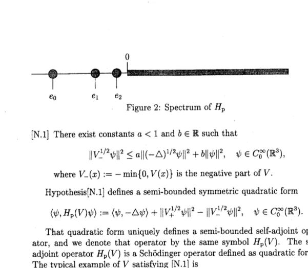
$e_{0}$ $e_{1}$ $e_{2}$

Figure 2: Spectrum of$H_{\mathrm{p}}$

[N.1] There exist constants $a<1$ and $b\in \mathbb{R}$ such that

$||V_{-}^{1/2}\psi||^{2}\leq a||(-\triangle)^{1/2}\psi||^{2}+b||\psi||^{2}$, $\psi$ $\in C_{0}^{\infty}(\mathbb{R}^{3})$,

where $V_{-}(x):=- \min\{0, V(x)\}$ is the negative part of$V$.

Hypothesis[N.l] defines

a

semi-bounded symm etric quadratic form

$\langle\psi$,$H_{\mathrm{p}}(V)\psi\}:=\langle\psi, -\triangle\psi\rangle+||V_{+}^{1/2}\psi||^{2}-||V_{-}^{1/2}\psi||^{2}$ , $\psi$

$\in C_{0}^{\infty}(\mathbb{R}^{3})$.

That quadratic form uniquely defines

a

semi-bounded self-adjoint

oper-ator, and we denote that operator by the

same

symbol $H_{\mathrm{p}}(V)$. The

self-adjoint operator $H_{\mathrm{p}}(V)$ is

a

Schodinger operator defined

as

quadratic forms.

The typical example of $V$ satisfying [N.1] is

$\mathrm{V}\{\mathrm{x})=-C/|x|$, $V(x)$ $=Cx^{2}$, $(C>0)$.

In the first(Coulomb) case, it iswell known that $H_{\mathrm{p}}$has negative eigenvalues

$\{e_{n}\}_{n=0}^{\infty}$ and $\sigma(H_{\mathrm{p}})=\{e_{n}\}_{n=0}^{\infty}\cup[0, \infty)$ (Figure 2).

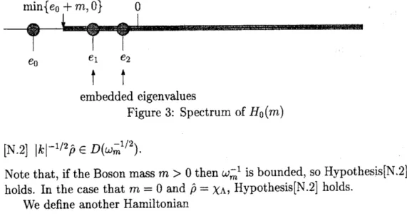
We call

$H_{0}(m):=H_{\mathrm{p}}$(&I$+\mathrm{n}$ (&$H_{\mathrm{b}}(m)$,

the free Hamiltonian. $H_{0}(m)$ does not include the interaction term between

the particle and the Bose field. Therefore

we can

find spectrum of $H_{0}(m)$

easily:

$\sigma(H_{0}(m))=\{\lambda+\mu\in \mathbb{R}|\lambda\in\sigma(H_{\mathrm{p}}), \mu\in\sigma(H_{\mathrm{b}}(m))\}$

$\sigma_{p}(H_{0}(m))=\{\lambda+\mu\in \mathbb{R}|\lambda\in\sigma_{p}(H_{\mathrm{p}}), \mu\in\sigma_{p}(H_{\mathrm{b}}(m))\}=\sigma_{p}(H_{\mathrm{p}})$.

In the Coulomb case,

we

draw $\sigma(H_{0}(m))$ at Figure 3.

The Hamiltonian of the standard Nelson model $H_{m}^{V}$ has the following

three parts:

$H_{m}^{V}:=H_{\mathrm{p}}(V)\otimes \mathrm{I}$ $+$ II(&$H_{\mathrm{b}}(m)$ $+\phi^{\oplus}(v)$.

thesecond term$H_{\mathrm{b}}(m)$ is the freeBoson Hamiltonian withBoson

mass

$m$,

and the last term $\phi^{\oplus}(v)$ is the interaction Hamiitonian between the particle

embedded eigenvalues

Figure 3: Spectrum of$H_{0}(m)$

[N.2] $|k|^{-1/2}\hat{\rho}\in D(\omega_{m}^{-1/2})$

.

Note that, if the Boson

mass

$m>0$ then$\omega_{m}^{-1}$ is bounded,

so

Hypothesis[N.2]

holds. In the

case

that $m=0$ and $\hat{\rho}=\chi_{\Lambda}$, Hypothesis[N.2] holds.

We define another Hamiltonian

$\tilde{H}_{m}^{V}:=H_{\mathrm{p}}(V)\otimes \mathrm{I}$$+\mathrm{I}$ (&$H_{f}(m)+\phi^{\oplus}(G)-\mathcal{V}_{m}(\hat{x})\otimes \mathrm{I}$$+\mathcal{W}_{m}\mathrm{I}$, (3) where $G(x, k):=v(x, k)-v(0, k)\in L^{2}(\mathbb{R}^{3})\cap D(|k|^{-1/2})$, $\mathcal{V}_{m}(\hat{x})$ is the

multi-plication operator by the function

$\mathcal{V}_{m}(x):={\rm Re}\langle\omega_{m}^{-1/2}v(0),\omega_{m}^{-1/2}v(x)\rangle$ ,

and $\mathcal{W}_{m}:=||\omega_{m}^{-1/2}v(\mathrm{O})||^{2}$ is

a

constant (note that, by [N.2], $v(x)$,$v(0)\in$ $D(\omega_{m}^{-1/2}))$.

The Hamiltonian of the quantumsystem must be self-adjoint. About the

Nelson model,

we can

easily prove the self-adjointness of these Hamiltonian:

Proposition 1.1. Assume that [N. 1] and [N.2]. Then $H_{m}^{V}$ and $\tilde{H}_{m}^{V}$ is

self-adjoint

on

$D$($H_{\mathrm{p}}\otimes \mathrm{n}$$+$ It$\otimes H_{\mathrm{b}}(m)$) and bounded below. Moreover $H_{m}^{V}$ and

$\tilde{H}_{m}^{V}$ is essentially self-adjoint

on

any

core

for

$H_{\mathrm{p}}$(&

$\mathrm{I}$$+\mathrm{I}$$\otimes H_{\mathrm{b}}(m)$.

Definition 1.2. We saythat the

_infrared

regular condition holds

if

and only

if

$|k|^{-1/2}\hat{\rho}\in D(\omega_{m}^{-1})$,

and

we

say that the

_infrared

singular condition holds

if

and only

_if

$|k|^{-1/2}\hat{\rho}\not\in D(\omega_{m}^{-1})$,

When the massive

case

$m>0$, $\omega_{m}^{-1}$ is bounded,

so

the infrared regular

condition holds. In the

case

$m=0$ and $\hat{\rho}=\chi_{\Lambda}$, it is easy to

see

that

$|k|^{-1/2}|k|^{-1}\chi_{\Lambda}\not\in L^{2}(\mathbb{R}^{3})$,

so

this

case

is

infrared

singular.

The following proposition

means

that infrared regular condition lead to

Proposition 1.3. Assume [N.1] and [N.2]. Suppose that the

infrared

regular

condition holds. Then the Hamiltonian $H_{m}^{V}$ is unitarily equivalent to $\tilde{H}_{m}^{V}$.

Proof.

By the infrared regular condition, the operator $T_{m}:=\exp[-\mathrm{i}\mathrm{N}\otimes$

$\Phi_{S}(\mathrm{i}v(0)/\omega_{m})]$ is

a

unitary operator

on

$\mathcal{F}$, and we have

$T_{m}H_{\mathrm{b}}(m)T_{m}^{*}=H_{\mathrm{b}}(m)-\mathbb{I}$$\otimes\Phi s(v(0))+\frac{1}{2}\langle v(0), \omega_{m}^{-1}v(0)\rangle$,

$T_{m}\phi^{\oplus}(v)T_{m}^{*}=\phi^{\oplus}(v)+{\rm Re}\langle\omega_{m}^{-1}v(0), v(x)\rangle$,

where we

use

a formula(see [2, Lemma 4-44 and $12rightarrow 5]$). Obviously $T_{m}$

com-mutes $H_{\mathrm{p}}$. Therefore $\tilde{H}_{m}^{V}=T_{m}H_{m}^{V}T_{m}^{*}$ .

$\mathrm{I}$

For $\Psi\in D(H_{\mathrm{b}}(m))$,

we

define

a

Fock space valued function $a(k)\Psi$ by

$a(k)\Psi=(\Psi^{(1)}(k), \sqrt{2}\Psi^{\langle 2)}(k, \cdot), \ldots, \sqrt{n}\Psi^{(n\}}\langle k, \cdot)$ ,

$\ldots$).

Next

we

define a distribution

on

the Fock space $\mathcal{F}_{\mathrm{b}}$ by

$(a(k)^{*} \Psi)^{\langle n)}:=\frac{1}{\sqrt{n}}\sum_{j=1}^{n}\delta(k-k_{j})\Psi^{(n-1)}(k_{1}, \ldots, k_{j-1}, k_{j+1}, \ldots, k_{n})$.

Here$\delta$ is theDiracdeltafunction. Thea$(k)’ \mathrm{s}$ and$a(k)^{*}’ \mathrm{s}$satisfythe following

’formal’ CCR relations:

$[a(k), a(k’)^{*}]=\delta(k-k’)$,

$[a(k), a(k’)]=[a(k)^{*}, a(k’)^{*}]=0$.

we

define

$b(k):=a(k)- \frac{1}{\sqrt{2}}\omega_{m}(k)^{-1}v(0, k)$,

$b(k)^{*}:=$

a

$(k)^{*}- \frac{1}{\sqrt{2}}\omega_{m}(k)^{-1}v(0, k)$.

The second term of$b(k)$, $b(k)$’ is constant foreach $k\in \mathbb{R}^{3}$

.

Hence $b(k)’ \mathrm{s}$ and

$b(k)^{*}’ \mathrm{s}$ satisfy the formal

CCR

relations:

$[b(k), b(k’)^{*}]=\delta(k-k’)$,

$[b(k), b(k’)]=[b(k)^{*}, b(k’)^{*}]=0$.

By using $a(k)$,

we

write the Hamiltonian $H_{m}^{V}$

as

$\langle\Psi, H_{m}^{V}\Psi\rangle=\langle\Psi, H_{\mathrm{p}}\otimes \mathrm{X}\Psi\rangle$ $+ \oint_{\mathbb{R}^{3}}\omega_{m}(k)\langle$$\mathrm{I}\otimes a(k)\Psi$, I$\otimes a(k)\Psi\rangle$$\mathrm{d}k$

and $\overline{H}_{m}^{V}$

can

be written

as

$\langle\Psi,\tilde{H}_{m}^{V}\Psi\rangle=\langle\Psi, H_{\mathrm{p}}\otimes 1\Psi\rangle$$+ \int_{\mathbb{R}^{3}}\omega_{m}(k)\langle \mathbb{I}\otimes b(k)\Psi, 1 \otimes b(k)\Psi\rangle \mathrm{d}k$

$+ \int_{\mathbb{R}^{3}}\frac{\hat{\rho}(k)}{|k|^{1/2}}[\langle e^{-ik\hat{x}}\otimes b(k)\Psi, \Psi\rangle+\langle\Psi, e^{-ik\hat{x}}\otimes b(k)\Psi\rangle]\mathrm{d}k$,

$a(k)$,$a(k)$’ is called the Fock representation of the

CCR.

When the

in-frared regular condition holds, $b(k)$,$b(k)^{*}$ is unitarily equivalent to the Fock

representationofthe CCR, but in the infrared singular case, $b(k)$,$b(k)^{*}$ is not

unitarily equivalent to the Fock representation of the CCR(see [2, p.202]).

By this reason, when the infrared singular condition holds, we call that the

operator $\tilde{H}_{0}^{V}$ is the Nelson Hamiltonian in

a

non-Fock representation.

2

Existence

of

Ground

State

Let $H$ be self-adjoint and bounded from below. We call the real value

$\mathrm{E}\mathrm{O}(\mathrm{H})=$ $\mathrm{a}(\mathrm{H})$ the ground (state) energy of $H$. If $E_{0}(H)$ is

an

eigen-value of$H$, the corresponding eigenvector is called

a

ground stateof$H$

.

We

set

$E^{V}(m):= \inf$a$(H_{m}^{V})$, $\tilde{E}^{V}(m):=\inf$

a

$(\overline{H}_{m}^{V})$

the ground state

energy

of$H_{m}^{V}$ and $\overline{H}_{m}^{V}$ respectively.

Proposition 2.1. Assume $[NJ]$ and [N.2]. Then

$E^{V}(m)=\tilde{E}^{V}(m)$

for

all$m\geq 0$.

Proof.

In the

case $m>0$

, by Proposition 1.3, $H_{m}^{V}$ is unitarily

equiva-lent to $\tilde{H}_{m}^{V}$. Hence $E^{V}(m)=\overline{E}^{V}(m)$ for $m>0$. Let

$m>m’>0$

,

then we have $H^{V}(m)$ $\geq H^{V}(m’)\geq H^{V}(0)$. Therefore, by the variational

principle $E^{V}(m)\geq E^{V}(m’)\geq E^{V}(0)$

.

Hence $\lim_{marrow+0}E^{V}(m)$ exists, and

$\lim_{marrow+0}E^{V}(m)\geq E^{V}(0)$. It iseasyto

see

that $\lim_{marrow+0}H_{m}^{V}\Psi=H_{0}^{V}\Psi$ for all $\Psi\in D(H_{\mathrm{p}})\otimes D(H_{\mathrm{b}}(\wedge 0))$, where $\otimes\wedge$

means

algebraic tensor product. Therefore

$H_{m}^{V}$ converges to $H_{0}^{V}$ in the strong resolvent

sense.

([9, Theorem VIIL25]).

Similarly $\overline{H}_{m}^{V}$

converges

to $\tilde{H}_{0}^{V}$ strong resolvent

sense.

Hence

we

have the

inverse inequality $\lim_{marrow+0}E^{V}(m)\leq E^{V}(0)$ and _{$\lim_{marrow+0}\overline{E}^{V}(m)\leq\tilde{E}^{V}(0)1$}

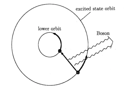
Figure

4:

All excited states

are

unstable

The problem

we

consider here is

Problem. Do $H_{m}^{V}$ and $\tilde{H}_{m}^{V}$ have

a

ground state?

In the

case

$m>0$, the free Hamiltonian$H_{0}(m)$ has

a

discrete groundstate

(see Figure 3). Therefore by the regular perturbation theory, the massive

Hamiltonian $H_{m}^{V}(m>0)$ has a ground state for sufficiently small $||\hat{\rho}||$. But

we

show that the massive(m $>0$) Hamiltonian $H_{m}^{V}$ has

a

ground state for all

coupling constant $||\hat{\rho}||$. In the proof about existence ofmassive ground state,

we

use

a localization estimate techniquewhich is developed by M. Griesemer,

E. Lieb, and M. Loss [4]. The condition to have a ground state

we

give here

is essentially

same

as GLL criterium[4], but

our

condition contains the

case

ofthe oscillator(V $=Cx^{\alpha}$, ($C$,$\alpha>0$)).

In the massless

case

$m=0$, alleigenvalueofthefree Hamiltonian$H_{0}(m=$

$0)$ embedded in the continuum(Figure 3),

so we can

not apply the regular

perturbation theory for any perturbation.

Since

the embedded eigenvalue

may vanish by

any

small perturbation, the analysis ofground state for $H_{0}^{V}$,

$\overline{H}_{0}^{V}$ is difficult.

When there is

no

interaction between the Bose field and the particle, all

excitedstates

are

stable becausethey

are

eigenvectorsofthefree Hamiltonian

$H_{0}(m=0)$. However, when the particle interact with the Bose field, the

excitedstate particleshouldemit

a

Boson and fallto

a

lower orbit (see Figure

4). Actually, in

an

atom, any excitedstate electronemits light spontaneously

and falls to

a

lower orbit. Namely, all excited states should be unstable.

state energy.

Incidentally, for

a

natural potential $V$, 1 believe that the Hamiltonian

$H_{0}^{V}$ and $\tilde{H}_{0}^{V}$ have

no

singular continuous spectrum. Then all spectrum of

the Hamiltonian is absolutely continuous spectrum if the Hamiltonian has

no

ground state. In this situation, for any state $\Psi\in \mathcal{F}$, the time evolution

of $\Psi$ converge weakly to

0

by the Riemann-Lebesgue Theorem, which is

a

contradiction. Because, the particle must remain

near

the origin

as

Figure

4.. Therefore ifthe particleHamiltonian $H_{\mathrm{p}}$hasground state andthe Nelson

modelisphysicallynatural, theHamiltonian oftheNelson model should have

a

ground state.

In 2001, A. Arai showed that the Nelson Hamiltonian in a non-Fock

rep-resentation $\tilde{H}_{0}^{V}$ has

a

ground state, if $V(x)\geq c|x|^{\alpha}$, $c$,$\alpha-2\geq 0$ and the

infrared singular condition holds(see[l]).

However, J. Lorinczi, R. A. Minlos and H. Spohn showed that if$V(x)\geq$

$c|x|^{a}$, $c$,

a–2

$\geq 0$ then the standard massless Nelson Hamiltonian $H_{0}^{V}$ has

no

ground state in the infrared singular case([7]).

In Mathematically, the existence of ground state is a phenomenon

de-pending

on

the representation ofthe CCR. In the context of this article, in

the infrared singular case, the Arai’s Nelson Hamiltonian $\tilde{H}_{0}^{V}$ is physically

natural

more

than the standard Nelson Hamiltonian $H_{0}^{V}$.

Let $\theta\in C_{0}^{\infty}(\mathbb{R}^{3}),\tilde{\theta}\in C^{\infty}(\mathbb{R}^{3})$ be functions which satisfy the following

properties (i), (ii):

(i) $0\leq\theta(x),\tilde{\theta}(x)\leq 1$, $\theta(x)^{2}+\overline{\theta}(x)^{2}=1$, $x\in \mathbb{R}^{3}$

.

(ii) $\theta(x)=\{$1,

$|x|\leq 1$,

0, $|x|\geq 2$

.

For $R>0$

we

define particle cutofffunctions $\theta_{R},\tilde{\theta}_{R}$

as

follows:

$\theta_{R}(x):=\theta(x/R)$, $\tilde{\theta}_{R}(x):=\theta(x/R)$.

We abbreviate $\theta_{R}\otimes \mathrm{I},\tilde{\theta}_{R}\otimes \mathrm{n}$ to $\theta_{R},\tilde{\theta}_{R}$

.

We define a minimal energy in the

state where the particle is separated

more

than $R$ away from the origin:

$E_{\infty}(R, m):= \Psi_{\frac{\in}{\theta}}Q(H_{m}^{V})\}|\inf_{R^{\Psi||\neq 0}}\frac{\langle\overline{\theta}_{R}\Psi,H_{m}^{V}\overline{\theta}_{R}\Psi\rangle}{||\overline{\theta}_{R}\Psi||^{2}},\tilde{E}_{\infty}(R, m):=\Psi Q(_{m^{)}}11_{R^{\Psi||\neq}}^{\frac{\in}{\theta}}\mathrm{i}\mathrm{n}_{\frac{\mathrm{f}}{H}\mathrm{v}_{0}}\frac{\langle\overline{\theta}_{R}\Psi,\tilde{H}_{m}^{V}\tilde{\theta}_{R}\Psi\rangle}{||\overline{\theta}_{R}\Psi||^{2}}$ ,

where $Q$

means

the form domain. Note that $E_{\infty}\underline{(}R$,$m$) and

$\overline{E}_{\infty}(R, m)$

are

have $E_{\infty}(R, m)$ $=\tilde{E}_{\infty}(R, m)$. By the variational principle,

we

have

$E_{\infty}(R, m)\geq E^{V}(m)$, $\tilde{E}_{\infty}(R, m)\geq\tilde{E}^{V}(m)$,

for all $m\geq 0$

.

Definition 2.2 (binding condition). We say the inequality

$E^{V}(m)< \lim_{R\prec}\sup_{\infty}E_{\infty}(R, m)$

the binding condition.

Now

we

state that the existence theorem ofthe massive Nelson model;

Theorem

2.3

(Existence ofground state $(m>0)$). Let$m>0$.

Assume

that

[N. 1] and $[N.2]$ hold. Suppose that the binding condition

for

$m>0$ holds.

Then $H_{m}^{V}$ has

a

groundstate.

Proof.

This proof is based

on

[4]. In this proof,

we

take the space

represen-tation for the Bosons. Namely,

we

consider

$\hat{H}:=\mathrm{I}\otimes\Gamma(\mathcal{F}^{-1})H_{m}^{V}$I$\otimes\Gamma(\mathcal{F})$

$=H_{\mathrm{p}}\otimes \mathrm{n}$$+\mathrm{n}$$\otimes \mathrm{d}\Gamma_{\mathrm{b}}(\sqrt{-\triangle+m^{2}})+\phi^{\oplus}(\mathcal{F}^{-1}v)$,

where $\mathcal{F}$ is the Fourier transform

on

the

one

Boson space, $\Gamma$ is the second

quantizationofsecond type, $\mathrm{d}\Gamma_{\mathrm{b}}$is thesecond quantizationoperator (see [2]),

and

$( \mathcal{F}^{-1}v)(x, y)=\frac{1}{(2\pi)^{3}}\int_{\mathbb{R}^{3}}\frac{\hat{\rho}(k)}{|k|^{1/2}}e^{-ik(x-y\}}\mathrm{d}k$,

where $x$ is the coordinate of the particle, and $y$ is the coordinate of the

Boson. For $P>0$

we

set $j_{1}(y):=\theta(y/P)$, $i_{2}(y):=\tilde{\theta}(y/R)$ the Boson cutoff

functions. We define

a

new

creation and annihilation operators

$c(f):=a(j_{1}f)\otimes 1$$+\mathrm{I}$$\otimes a(j_{2}f)\}$

$c(g)^{*}:=a(j_{1}g)^{*}\otimes 1$ $+\mathrm{I}$

&

$a(j_{2}g)^{*}$, $f$,$g\in L^{2}(\mathbb{R}^{3})$,

which is

a

closed operator

on

$\mathcal{F}_{\mathrm{b}}\otimes \mathcal{F}_{\mathrm{b}}$. Let

$\mathcal{F}_{\ell}:=\overline{\mathcal{F}_{\ell,\mathrm{f}\mathrm{i}\mathrm{n}}}\subseteq \mathcal{F}_{\mathrm{b}}\otimes \mathcal{F}_{\mathrm{b}}$,

$\mathcal{F}_{\ell,\mathrm{f}\mathrm{i}\mathrm{n}}:=\mathcal{L}\{\Omega\otimes\Omega, c(g_{1})^{*}\cdots c(g_{k})^{*}\Omega\otimes\Omega|g_{j}\in L^{2}(\mathbb{R}^{3}),j=1_{7}\ldots, k, k\in \mathrm{N}\}$.

We define

a

operator $U_{0}$ : $\mathcal{F}_{\mathrm{b}}arrow \mathcal{F}_{\mathrm{b}}\otimes \mathcal{F}_{\mathrm{b}}$ by

$D(U_{0}):=\mathcal{F}_{\mathrm{f}\mathrm{i}\mathrm{n}}$,

where $\mathcal{F}_{\mathrm{f}\mathrm{i}\mathrm{n}}$

means

the finite particle subspace (see [2]). It iseasy to see that

$U_{0}$ is isometry, and $U:=\overline{U_{0}}$ is isometric operator from $\mathcal{F}_{\mathrm{b}}$ to $\mathcal{F}_{\mathrm{b}}\otimes \mathcal{F}_{\mathrm{b}}$ with

Ran(U) $=\mathcal{F}_{\ell}$. Therefore

$U^{*}U=\mathrm{I}_{F_{\mathrm{b}}}$, $UU^{*}=$ orthogonal projection

on

$\mathcal{F}_{\ell}$.

We define adense space by $V$ $:=C_{0}^{\infty}(\mathbb{R}^{3})\otimes \mathcal{F}_{\mathrm{f}\mathrm{i}\mathrm{n}}(C_{0}^{\infty}(\mathbb{R}^{3})\wedge)$. By the IMS

local-ization formula, we have that

$\hat{H}=\theta_{R}\hat{H}\theta_{R}+\tilde{\theta}_{R}\hat{H}\tilde{\theta}_{R}-\frac{1}{2}|\nabla\theta_{R}|^{2}-\frac{1}{2}|\nabla\tilde{\theta}_{R}|^{2}$ , (4)

in the

sense

of quadratic form

on

$\prime D$. The key of the proof is the following

lemma

Lemma 2.4. For all $\Psi\in D_{f}$ we have that

$\langle\Psi, \theta_{R}\hat{H}\theta_{R}\Psi\rangle=\langle\Psi, \theta_{R}U^{*}\{\hat{H}\otimes \mathrm{I}_{\mathcal{F}_{\mathrm{b}}}+1_{F}\otimes H_{\mathrm{b}}(m)\}U\phi_{R}\Psi\rangle$

$+o(1)\langle\Psi, (\hat{H}-E^{V}(m)+1)\Psi\rangle$,

in the

sense

_of

quadratic form, where the operator in $\{\}$ is acting on the

Hilbert space$\mathcal{F}\otimes \mathcal{F}_{\mathrm{b}}$, and$o(1)$ is a constant such that$\lim_{Rarrow\infty}\lim_{Parrow\infty}o(1)=$

$0$

.

We omit the proof of this Lemma(see [4]). By this lemma and (4),

we

have

$\hat{H}\geq\theta_{R}U^{*}\{E^{V}(m)\otimes \mathrm{I} +\mathrm{n} (\otimes m(1 -P_{2})\}U\theta_{R}$

$+E_{\infty}(R,m)\overline{\theta}_{R}^{2}+o(1)$(ff $-E^{V}(m)+1$),

in the

sense

ofquadratic form

on

$\prime D$, where $P_{2}$ is the orthogonal projection

on

Q. _Therefore

$\hat{H}-E^{V}(m)\geq(E_{\infty}(R, m)-E^{V}(m))\theta_{R}^{\tilde{2}}+m\theta_{R}^{2}-m\theta_{R}U^{*}I\otimes P_{2}U\theta_{R}$

$+o(1)(\hat{H}+\mathrm{I})$

.

Note that $T$ $:=\theta_{R}U^{*}1\otimes P_{2}U\theta_{R}=(\Gamma(j_{1})\theta_{R})^{2}$

.

Since

$H_{\mathrm{b}}(m)$ is massive, hence

$T$ is ($-\triangle\otimes$ II $+\mathrm{I}$ $\otimes H_{\mathrm{b}}(m)+1$)-form compact(more precisely

see

[4]). By

$\theta_{R}^{2}+\theta_{R}^{\tilde{2}}=1$,

we

have that

$(E_{\infty}(R, m)-E^{V}(m)) \theta_{R}^{\tilde{2}}+m\theta_{R}^{2}\geq\min\{E_{\infty}(R, m)-E^{V}(m), m\}$.

Therefore

we

get

in the

sense

of the quadratic form

on

$Q(\hat{H})$, where

we

done the closed

ex-tension of the quadratic form. Using the condition $[\mathrm{N}.\mathrm{I}],[\mathrm{N}.2]$,

one can

show that $T$ is $\hat{H}$ -form compact. So _$T$ does not change the essential spectrum of

$H_{\ovalbox{\tt\small REJECT}}$ and hence

$(1-o(1)) \Sigma(\hat{H})-E^{V}(m)\geq\min E_{\infty}(R, m)-E^{V}(m)$,$m+o(1)$, (5)

where $\Sigma$

means

the bottom ofthe essential spectrum. Now

we

take the limit

$\lim_{Rarrow\infty}\lim_{Parrow\infty}$, and

we

get

$\Sigma(\hat{H})-E^{V}(m)>0$.

This inequality

means

that $\hat{H}$ has

a

discrete ground state.

1

For existence of the massless ground state,

we

assume

these following

conditions:

[N.3] There exists

an

open set $S\subset \mathbb{R}^{3}$, such thattt $\mathrm{s}\mathrm{u}\mathrm{p}\mathrm{p}/5=\overline{S}$. Moreover, for

all $n\in \mathrm{N}$

$S_{n}:=\{\mathrm{i}\in S||k|<n\}$

has the cone-property (see [6]).

[N.4] There exists a function y7 $\in H^{1}(\mathbb{R}^{3})$, such that $\hat{\rho}=\chi s\eta$.

[N.5] $\hat{\rho}$ is continuously differentiate in $S\backslash \{0\}$.

[N.6] $|k|^{-3/2}\hat{\rho}$, $|k|^{-1/2}|\nabla\hat{\rho}|\in L^{p}(S)$ for all $p\in(1,2)$.

Theorem 2.5 (Existence of ground state $m=0$). Let $m=0$. Assume

conditions$fN.l$]$-[N.\theta]$

.

If

the binding condition holds, then $\tilde{H}_{0}^{V}$ has a ground

state.

Remark. If$\lim$

}$x|arrow\infty V(x)=\infty$, one can show that $\lim_{Rarrow\infty}E_{\infty}(R, m)=\infty$.

Therefore the binding condition holds. If$\lim|x|arrow\infty V(x)$ $=0$, $V\in L_{1\mathrm{o}\mathrm{c}}^{2}(\mathbb{R}^{3})$ and $H_{\mathrm{p}}$ has

a

negative ground state. Then the binding condition holds (see

[4, Theorem 3.1]$)$

.

Remark. $\hat{\rho}=\chi_{\mathrm{A}}$ satisfies the conditions [N.$1$]$-[\mathrm{N}.6]$.

References

[1] A. Arai, Ground state of the massless Nelson model without infrared

cutoffin

a

non-Fock representation, Rev. Math. Phys. 9 (2001),

1075-191

[2] A. Arai, Fock spaces and Quantum fields (Nippon-Hyouronsya, Tokyo,

2000) (in Japanese).

[3]

C.

G\’erard, On the existence ofground states for massless Pauli-Fierz

Hamiltonians, Ann. Henri Poincare 1 (2000),

443-459.

[4] M. Griesemer, E. Lieb and M. Loss, Ground states in non-relativistic

quantum electrodynamics, Invent math. 145 (2001), 557-595.

[5] M. Hirokawa, F. Hiroshimaand H. Spohn, Ground states forpoint

par-ticles interacting through a massless scalar bose field, Adv. Math. 191

(2005), 339-392.

[6] E. H. Lieb, M. Loss, Analysis, Amer. Math. Soc. second edition, 2001.

[7] J. Lorinczi, R. A. Minlos and H. Spohn The infrared behaviour in

Nel-son’s model of

a

quantum particle coupled to a massless scalar field,

Ann. Henri Poincare 3 (2002), 269-295.

[8] E. Nelson, “Interaction of nonrelativistic particles with

a

quantized

scalar field”, J. Math. Phys. 5 (1964)

1190-1197.

[9] M. Reed and B. Simon, Methods ofModern Mathematical Physics Vol.

I, Academic Press, New York, 1972.

[10] M. Reed and B. Simon, Methods of Modern Mathematical Physics Vol.

II, Academic Press, New York,

1975.

[11] M. Reed and B. Simon, Methods ofModern Mathematical Physics Vol.

IV, Academic Press, NewYork,

1978.

[12] I. Sasaki, Ground state of the massless Nelson model in a non-Fock

representation, J. Math. Phys. 46, (2005)

[13] H. Spohn, Groundstates of

a

quantum particle coupled to a scalar bose