Presentations of (immersed) surface-knots by marked graph diagrams (Intelligence of Low-dimensional Topology)

全文

(1)98. 数理解析研究所講究録第2052巻 2017年 98-108. Presentations of. (immersed). surface‐knots. by. marked. graph. diagrams Jieon Kim. Osaka city. University /JSPS. Introduction. 1. An immersed. surface‐link. is. a. generically. \mathbb{R}^{4} When the surface has only. immersed closed oriented surface in the. component, it is also called. 4‐space. immersed. surface‐knot. When the surface consists of 2‐spheres, it is also called an immersed sphere‐link or simply an immersed 2‐link. When the immersion is an embedding, it is also called a surface‐link. Two (immersed) surface‐links \mathcal{L} and \mathcal{L}' are equivalent if there is an orientation‐preserving auto‐homeomorphism h of \mathbb{R}^{4} sending \mathcal{L} to \mathcal{L}' orientation‐preservingly. A normal form of an immersed surface‐link introduced by S. Kamada and K. Kawamura in [5] is used to define a marked graph diagram of an immersed surface‐link. In [6], we extend the method of presenting surface‐links by marked graph diagrams to presenting immersed surface‐links. We also give some local moves on marked graph diagrams that preserve the ambient isotopy classes of their presenting immersed surface‐links, which are extension of moves given by Yoshikawa [19] for presentation of embedded surface‐links. .. 2. Marked. In this. section,. we. vertex with. a. review. [6].. (oriented). A marked. marked. graph. marker looks like. is. \rangle\langle. .. a. an. of immersed surface‐links. graph representation. links described in a. one. graph diagrams representing immersed surface‐ graph in \mathbb{R}^{3} each of whose vertices is. 4‐valent. Two marked. graphs. are. said to be. equivalent. if. they are ambient isotopic in \mathbb{R}^{3} with keeping the rectangular neighborhoods of markers. As usual, a marked graph in \mathbb{R}^{3} can be described by a link diagram on \mathbb{R}^{2} with some 4‐ valent vertices equipped with markers, called a marked graph diagram. An orientation of a marked graph G in \mathbb{R}^{3} is a choice of an orientation for each edge of G An orientation of .. a. marked. graph G. graph. in. G is said to be consistent if every vertex in G looks like. \mathbb{R}^{3} is said. to be orientable if G admits. is said to be non‐orientable.. By. an. consistent orientation.. a. oriented marked. \geq $\xi$. graph. we mean an. .. A marked. Otherwise,. it. orientable marked. graph in \mathbb{R}^{3} with a fixed consistent orientation. Two oriented marked graphs are said to be equivalent if they are ambient isotopic in \mathbb{R}^{3} with keeping the rectangular neighbor‐ hood, marker and consistent orientation. For t\in \mathbb{R} we denote by \mathb {R}_{t}^{3} the hyperplane of \mathbb{R}^{4} whose fourth coordinate is equal to t\in \mathbb{R} i.e., \mathb {R}_{t}^{3} \{(x_{1}, x_{2}, x_{3}, x_{4}) \in \mathbb{R}^{4} | x_{4} =t\}. ,. ,. =.

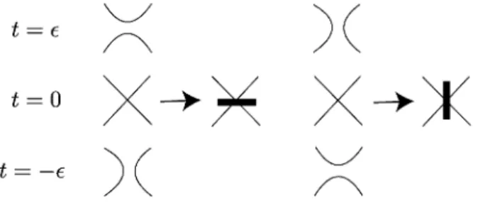
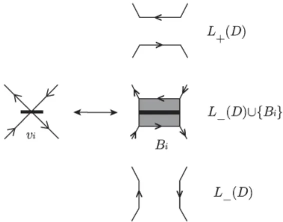
(2) 99. An immersed surface‐link \mathcal{L}\subset \mathbb{R}^{4}=\mathbb{R}^{3}\times \mathbb{R}. \mathcal{L}_{t}=\mathcal{L}\cap \mathbb{R}_{t}^{3},. t\in \mathbb{R}. (cf. [3]).. \mathcal{L}'\subset \mathbb{R}^{3}[-2, 2]. immersed surface‐link. (1). The intersections \mathcal{L} í and. (2). All saddle points of \mathcal{L}'. (3). All maximal points of \mathcal{L}'. (4). All minimal points of \mathcal{L}'. (5). normal. a. cones. form. .. illustrated in. \mathbb{R}^{3}[2] ;. in. \mathbb{R}^{3}[-2] ;. a. .. links;. \mathcal{L}'\cap(\mathbb{R}^{3}[-2, -1]) are disjoint unions of a disjoint disjoint system of Hopf link cones.. a. Let \mathcal{L} be. spatial. (saddle point). 1. We choose. an. and. and. of \mathcal{L}. \mathrm{H} ‐trivial. in. are. are. be described in terms of its cross‐sections. \mathbb{R}^{3}[0] ;. in. are. normal form of \mathcal{L} Then \mathcal{L} Ó is each 4‐valent vertex. are. \mathcal{L}'\cap(\mathbb{R}^{3}[1,2]). The intersections. system of trivial knot. We call \mathcal{L}'. \mathcal{L}_{-1}'. can. [5]. that any immersed surface‐link \mathcal{L} , there is satisfying the following conditions:. It is shown. an. 4‐valent. immersed surface‐link in \mathbb{R}^{4} , and \mathcal{L}'. regular graph. in. that indicates how the saddle. \mathb {R}_{0}^{3}. .. We. point. give. a. \mathrm{a}. marker at. opens up above. as. of \mathcal{L} Ó that coincides with the. orientation for each. edge boundary of \mathcal{L}'\cap \mathbb{R}^{3}\times(-\infty, 0 ] from the orientation of \mathcal{L}' The resulting oriented marked graph G is called an oriented marked graph of \mathcal{L} As usual, G is described by a link diagram D with rigid marked vertices. Such a diagram D is called an oriented marked graph diagram or an oriented ch‐diagram (cf. [17]) of \mathcal{L}. Fig.. induced orientation. on. an. the. .. .. Figure. 1:. Marking. of. a. vertex. an oriented marked graph diagram. We obtain two links L_{-}(D) and L_{+}(D) by replacing each marked vertex in D as shown in Fig. 2. Links L_{-}(D) and L_{+}(D) are also called the negative resolution and the positive resolution of D respectively. By replacing a neighborhood of each marked vertex v_{i} (1 \leq i \leq n) with an oriented band B_{i} as illustrated in Fig. 2. Denote the disjoint union B_{1}\sqcup\cdots\sqcup B_{n} of bands by \mathcal{B}(D) \mathrm{A} link L is \mathrm{H} ‐trivial if L is a split union of trivial knots and Hopf links. A marked graph diagram D is said to be \mathrm{H} ‐admissible if both resolutions L_{-}(D) and L_{+}(D) are \mathrm{H} ‐trivial classical link diagrams as shown in Fig. 3.. Let D be. from D. ,. .. From. given. now. on,. we. recall how to construct. \mathrm{H} ‐admissible oriented marked. oriented marked proper. surface. graph diagram.. associated with D ,. an. immersed surface‐link \mathcal{L} in \mathbb{R}^{4} from. graph diagram (cf. [5,. We define. by. a. surface‐link. 6. Let D be. an. a. \mathrm{H} ‐admissible. \mathcal{F}(D) \subset \mathbb{R}^{3}\times[-1, 1]. ,. called the.

(3) 100. 2: Marked vertex resolutions. Figure. Figure. 3: An \mathrm{H} ‐admissible marked. \left{\begin{ar y}{l (\mathb{R}^3,L_{+}(D)&\mathr {f}\mathr {o}\mathr {}0<t\leq1,\ (mathb{R}^3,L_{-}(D)\cup mathcl{B}(D)&\mathr {f}\mathr {o}\mathr {}t=0,\ (mathb{R}^3,L_{-}(D)&\mathr {f}\mathr {o}\mathr {}-1\leqt<0. \end{ar y}\ight.. (\mathbb{R}_{t}^{3}, \mathcal{F}(D)\cap \mathbb{R}_{t}^{3})= It is known that. \mathcal{F}(D). a. marked. graph diagram. associated with D is. the resolutions. L_{+}(D). and. an. graph diagram. D is orientable if and. orientable surface.. L_{-}(D). Since D has. .. We choose. a. have the orientations induced from the orientation of. orientation for the proper surface \mathcal{F}(D) of the cross‐section L_{+}(D) =\mathcal{F}(D)_{1} \mathcal{F}(D)\cap \mathbb{R}_{1}^{3} at t. D. if the proper surface consistent orientation,. only. an. =. that the induced orientation 1 matches the orientation of. be a closed interval with a<b For a link L let \hat{L}*[a, b] (or \check{L}*[a, b] ) L[a] (or L[b] ) as the base and a point in \mathbb{R}^{3}[b] (or \mathbb{R}^{3}[a] ), respectively. Let H=(O_{1}\cup\cdots\cup O_{m})\cup(P_{1}\cup\cdots\cup P_{n}) be an \mathrm{H} ‐trivial link in \mathbb{R}^{3} where O_{i} is a trivial knot and P_{j} is a Hopf link for i=1 n. m, j=1. L_{+}(D). be. Let. .. a cone. [a, b]. so =. .. ,. with. ,. ,. \bullet. 1, \bullet. H_{\wedge}[a, b]. Let .. .. .. ,. m). and. H_{\vee}[a, b]. Let 1,. .. .. .. ,. m). be. .. .. ,. ,. .. .. .. ,. disjoint union of a disjoint system of trivial knot cones \hat{O}_{i}*[a, b](i= disjoint system of Hopf link cones \hat{P}_{j}*[a, b](j=1, . . . , n) in \mathbb{R}^{3}[a, b].. a. a. be. and. .. disjoint union of a disjoint system of trivial knot cones \check{O}_{i}*[a, b](i= disjoint system of Hopf link cones \check{P}_{j}*[a, b](j=1, . . . , n) in \mathbb{R}^{3}[a, b].. a. a.

(4) 101. By capping off \mathcal{F}(D). mersed surface‐link oriented immersed struction of. surface‐link. S(D) S(D). with. S(D). L_{+}(D)_{\wedge}[1 2 ] ,. in. \mathbb{R}^{4}. an. oriented marked. D if \mathcal{L} is ambient. Theorem 2.2. Let \mathcal{L} be. graph diagram We discuss. we. obtain. an. oriented im‐. .. It is. S(D). the. .. Definition 2.1. An immersed surface‐link \mathcal{L} is. graph diagram. ,. straightforward from the con‐ graph diagram of the oriented immersed. associated with D. surface‐link. that D is. L_{-}(D)_{\vee}[-2, -1]. and. We call the oriented immersed surface‐link. .. an. to. presented by. S(D). an. presented by. an. graph diagrams which preserve the presented by the diagrams.. Figure. \mathrm{H} ‐admissible marked. D.. marked. of the immersed surface‐links. \mathrm{H} ‐admissible marked. constructed from D.. immersed surface‐link. Then there is. D such that \mathcal{L} is. moves on. isotopic. 4: Moves of. Type. ambient. isotopy classes. I. depicted in Fig. 4 on marked graph diagrams are called moves of type I, change the equivalence classes of marked graphs in \mathbb{R}^{3}. The moves depicted in Fig. 5 on marked graph diagrams are called moves of type II, which change the equivalence classes of marked graphs in \mathbb{R}^{3} When a marked graph D H is ‐admissible then the result obtained from D by any move diagram (or admissible) The. moves. which do not. .. of type II is also H ‐admissible (or admissible) and the immersed surface‐link link) presented by the diagrams are ambient isotopic, respectively. It is known that two admissible marked. surface‐links if and These. moves are. only. if. they. are. called Yoshikawa. related moves.. by. graph diagrams present. the. moves. of type I and II. (or. surface‐. ambinet. isitopic. (cf. [14, 18,. 19.

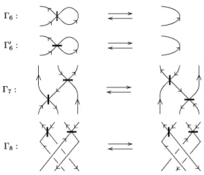
(5) 102. Figure. 5: Moves of. Type. II. Let D be a link diagram of an H ‐trivial link L A crossing point p of D is an unlinking crossing point if it is a crossing between two components of the same Hopf link of L and if the crossing change at p makes the Hopf link into a trivial link. .. Definition 2.3. Let D be. an H ‐admissible marked graph diagram and let D_{-} and D_{+} be diagrams of the lower resolution L_{-}(D) and the upper resolution L_{+}(D) respectively. A crossing point p of D is an lower singular point (or an upper singular point, respectively) if p is an unlinking crossing point of D_{-} (or D_{+} ).. the. ,. We introduce. new moves. for H ‐admissible marked. graph diagrams. They. are. the. moves. of type III. For the moves (a) of $\Gamma$_{9} and $\Gamma$_{9}' in $\Gamma$_{10} $\Gamma$_{9}, $\Gamma$_{9}' Fig. 6, we a condition that the 6 Fig. require components l^{+} (in the resolution L_{+}(D) ) and l^{-} (in the resolution L_{-}(D) ) are trivial, respectively. For the moves (b) of $\Gamma$_{9} and $\Gamma$_{9}' , we require and. a. in. condition that p is. an. which. we. call. upper. singular point. Figure. moves. and. 6: Moves of. a. lower. Type. III. singular point, respectively..

(6) 103. The. generalized. (Type I), $\Gamma$_{6}. ,. .. .. .. ,. Yoshikawa. moves. for marked. graph diagrams. $\Gamma$_{8} (Type II), and $\Gamma$_{9}, $\Gamma$_{9}', $\Gamma$_{10} (Type III). as. are. the. shown in. $\Gamma$_{1}. moves. ,. .. .. Fig. 4, Fig. 5,. .. ,. $\Gamma$_{5}. and. Fig. 6, respectively.. Definition 2.4. Let D and D' be marked. D'. are. stably equivalent. if. they. are. graph diagrams. Marked graph diagrams D and by a finite sequence of generalized Yoshikawa. related. moves.. Definition 2.5. A set S of. of. moves. in. S\backslash \{x\}. moves are. (S. Kamada,. Question. 2.6. Yoshikawa. moves. independent if x. is not. generated by finite. sequences. for every x\in S. A.. Kawauchi,. J.. Kim, S.. Y. Lee. [6]).. Is the set of. generalized. independent? surface‐links, and D and D' their marked are related by a finite sequence of general‐ equivalent.. Lemma 2.7. Let \mathcal{L} and \mathcal{L}' be immersed. graph diagrams, respectively.. If D and D'. ized Yoshikawa moves, then \mathcal{L} and \mathcal{L}' Problem 2.8. the marked are. (J. Kim).. are. Find the set S of local. graph diagrams equivalent.. are. related. by S. of marked. moves. if and. only. graph diagrams. such that. if their immersed surface‐links. (J. Kim). Create a table of \mathrm{H} ‐admissible marked graph diagrams repre‐ senting immersed surface‐links under the equivalence of S in the previous Problem with ch‐index 10 or less, where the ch‐index of a marked graph diagram is the sum of the number of crossings and that of vertices. Problem 2.9. Definition 2.10 (cf. [5]). A positive (or negative) standard singular 2‐knot, denoted is the immersed 2‐knot of the marked graph diagram D (or D' ) in by S(+) (or S Fig. 7, respectively. An unknotted immersed sphere is defined to be the connected sum mS(+)\# nS(-) for any non‐negative integers m, n with m+n>0.. A double point singularity p of of an immersed 2‐knot and. sum. the unknotted immersed. an. an. immersed 2‐knot S is inessential if S is the connected unknotted immersed. sphere. Otherwise,. D. Figure. sphere. p is essential.. 7: Standard. D'. singular. 2‐knot. such that p. belongs. to.

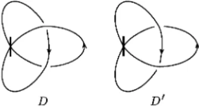
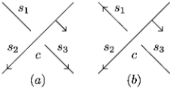
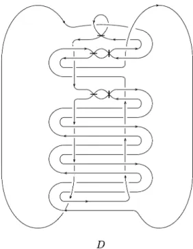
(7) 104. Confirming. 3. immersed 2‐knots with essential. singularity. an example of infinitely many singularity. For an immersed 2‐knot K let E(K) \mathrm{C}1(S^{4}\backslash \mathrm{N}(K)\mathrm{J} Let Ẽ(K) be the infinite cyclic covering of E(K) Then the homology H(K)=H_{1}(E(K)) is a finitely generated $\Lambda$ ‐module, where $\Lambda$=\mathbb{Z}[t, t^{-1}] This module is called the first Alexander module of K (cf. [15]). Let. In this. section, the. main theorem will be shown with. immersed 2‐knots with essential. =. ,. .. .. .. DH(K)= {x\in H(K)| \exists\{$\lambda$_{i}\}_{1\leq i\leq m} : coprime (m\geq 2) called the annihilator $\Lambda$ ‐submodule, which is known to be. part of the Alexander module. H(K) (cf. [9,. with. equal. $\lambda$_{i}x=0, \forall i },. to the. integral torsion elementary unchanged by replacing t by t^{-1}.. Section 3. Let. $\epsilon$(K). be the first. DH(K) A $\Lambda$ ‐ideal is symmetric if the ideal is DH(K)^{*}=\mathrm{h}\mathrm{o}\mathrm{m}(DH(K), \mathbb{Q}/\mathbb{Z}) have the induced $\Lambda$ ‐module structure, $\Lambda$ ‐module of DH(K) The following lemma is used in our argument.. ideal of. .. Let. called the dual. .. Lemma 3.1. If K is. DH(K). ,. a. then the first. 2‐knot such that the dual $\Lambda$ ‐module. elementary. ideal. $\epsilon$(K). is. DH(K)^{*}. is $\Lambda$ ‐isomorphic to. symmetric.. For any marked graph diagram D of K , the fundamental group $\pi$(K) of K is generated the connected components of D , namely, the connected components obtained from D. by by cutting. (a). or. (b). the in. under‐crossing points Fig. 8.. and the relations. (a) Figure. s_{3}=s_{2}^{-1}s_{1}s_{2}. for all. crossings. as. in. (b). 8: Labels at. crossing. a. A computation of the Alexander module example as follows:. H(K). or a. vertex. and the ideal. $\epsilon$(K). is shown in. a. concrete. Example 3.2. Let K be the immersed 2‐knot of D in Fig. 9. The immersed 2‐knot K only one double point. The fundamental group $\pi$(K) is computed as follows: $\pi$(K)=<x_{1},x_{2},x_{3},x_{4},x_{5},x_{6},x_{7},x_{8},x_{9},x_{10},x_{11},x_{12},x_{13},x_{14},x_{15}|x_{1}=x_{2}^{-1}x_{3}x_{2}, x_{2}=x_{3}^{-1}x_{5}x_{3}, x_{1}=x_{3}^{-1}x_{4}x_{3}, x_{2}= x_{1}^{-1}x_{3}x_{1},x_{6}=x_{2}^{-1}x_{1}x_{2}, x_{6}=x_{1}^{-1}x_{7}x_{1}, x_{1}=x_{7}^{-1}x_{8}x_{7}, x_{2}=x_{7}^{-1}x_{9}x_{7},x_{10}=x_{2}^{-1}x_{7}x_{2}, x_{10}=x_{1}^{-1}x_{11}x_{1}, x_{1}= x_{11}^{-1}x_{12}x_{11}, x_{2}=x_{11}^{-1}x_{13}x_{11},x_{14}=x_{2}^{-1}x_{11}x_{2}, x_{14}=x_{1}^{-1}x_{2}x_{1},x_{1}=x_{2}^{-1}x_{15}x_{2}>. has. This group. $\pi$(K) r_{1}. Then the. is :. following. isomorphic. to the group <x_{1},. x_{2}x_{1}x_{2}^{-1}=x_{1}x_{2}x_{1}^{-1}. ,. r_{2}. :. x_{2}|r_{1}, r_{2}>. ,. where. (x_{1}x_{2}^{-1})^{3}x_{1}(x_{1}x_{2}^{-1})^{-3}=x_{2}.. $\Lambda$ ‐semi‐exact sequence. $\Lambda$[r_{1}^{*}, r_{2}^{*}]^{d}-3 $\Lambda$[x_{1}^{*}, x_{2}^{*}]4^{d} $\Lambda$\rightar ow $\epsilon$ \mathbb{Z}\rightar ow 0 of the group presentation of $\pi$(K) is obtained by using the fundamental formula of the Fox differential calculus in [1], where $\Lambda$[r_{1}^{*}, r_{2}^{*}] and $\Lambda$[x_{1}^{*}, x_{2}^{*}] are free $\Lambda$ ‐modules with bases.

(8) 105. r_{i}^{*}. (i= 1,2). given. as. x_{j}^{*} (j = 1,2) respectively,. and. ,. follows:. and the $\Lambda$ ‐homomorphisms $\epsilon$,. d_{1} and d_{2}. are. $\epsilon$(t)=1, d_{1}(x_{j}^{*})=t-1(j=1,2) , d_{2}(r_{i}^{*})=\displaystyle \sum_{j=1}^{u}\frac{\partial r_{i} {\partial x_{j} x_{j}^{*}(i=1,2) for the Fox differential calculus. regarded. Theorem. element of $\Lambda$. by letting x_{j}. =. matrix of the $\Lambda$ ‐homomorphism. presentation. as an. to t. .. The. H(K) is identified with the quotient $\Lambda$ ‐module \mathrm{K}\mathrm{e}\mathrm{r}(d_{1})/{\rm Im}(d_{2}) (see 7.1.5]). The Alexander matrix M_{K} (m_{ij}) defined by m_{ij} \displayt e\frac{prtial_{}\partilx_{j} is a. Alexander module. [10,. \displayt e\frac{prtial_{}\partilx_{j}. =. d_{2} and calculated. as. follows:. M_{K}= \left\{\begin{ar ay}{l } 2t-1 & 1-2t\ 4-3t & 3t-4 \end{ar ay}\right\} Hence. we. have. H(K)\cong $\Lambda$/(2t-1,4-3t) which is. equal. to. DH(K) Thus,. the first. .. elementary. ,. ideal. $\epsilon$(K). of K is. $\epsilon$(K)=<2t-1, 4-3t> =<2t-1, 4-3t, 3(2t-1)+2(4-3t)> =<2t-1, 5>. The. lemma is useful in. following. ([13]). Lemma 3.3. 1. The ideal 2. An. following. statements. are. a. symmetric ideal.. equivalent:. <2t-1, m>\mathrm{i}\mathrm{s} symmetric.. integer. m. is \pm 2^{r}. ([13]). Lemma 3.4.. The. computation for. a. or. There. \pm 2^{r}3 for any. are. infinitely. integer r\geq 0.. many immersed 2‐knots with. one. essential double. point singularity. Let J be. one. of the immersed 2‐knots. $\epsilon$(J). elementary. ideal. Corollary. 3.5. The connected. |DH(J)|. group orders. essential double. Finally,. By using. [4].. an. K_{m}^{*}. sum. |DH(U)|. J#U of J and are coprime is. (2t- 1,5). any immersed 2‐knot U such that the immersed 2‐knot with at least one. an. is known to be the first. immersed 2‐knot in Lemma. Theorem 3.6. 2‐knot. asymmetric.. and. K_{n}, K_{n}' (n = 1,2,3, \ldots) such that the first following corollary is obtained.. Then the. point singularity.. the ideal. torus‐knot in. is. with. ([13]) one. Let. K=nK_{m}^{*}. essential double. elementary. 3.4, the following. be the connected. point singularity. sum. ideal of. main theorem is. of. n. copies of. whose first. an. a. ribbon. proved. immersed. elementary. ideal is. for any integer m \geq 5 without factors 2 and 3. Then K gives infinitely many immersed 2‐knots with n double point singularities every of which is essential. <. 2t-1, m. >.

(9) 106. D. Figure. 9: An \mathrm{H} ‐admissible marked. graph diagram. D. References. [1]. R. H. Crowell and R. H. FOX: Introduction to Knot. Mass.,. [2]. Theory, Ginn. and. Co., Boston,. 1963.. M. S. Farber:. Duality. Math.USSR‐Izv. 11. in. (1977),. an. infinite cyclic covering. and even‐dimensional. knots,. 749‐781.. [3]. R.H. Fox:. [4]. F. Hosokawa and A. Kawauchi:. A quick trip through knot theory, Toplogy of 3‐manifolds and Related Topics, (Prentice‐Hall, Inc., Englewood Cliffs, N.J., 1962), 120‐167.. J. Math. 16. (1979),. Proposals for. unknotted. surfaces. in. four‐space, Osaka. 233‐248.. [5]. S. Kamada and K. Kawamura:. [6]. S.. [7]. S. Kamada and K. Kawamura, Ribbon‐clasp surface‐links and normal forms of gular surface‐links, Topology Appl, to appear, ArXiv: 1602. 07855vl.. Ribbon‐clasp surface‐links and normal forms of gular surface‐links, Topology Appl. (to appear), arXiv:1602.07855. Kamada, A. Kawauchi, J. Kim, surface‐link (preprint).. and S. Y. Lee:. Marked. sin‐. graph diagrams of. an. immersed. sin‐.

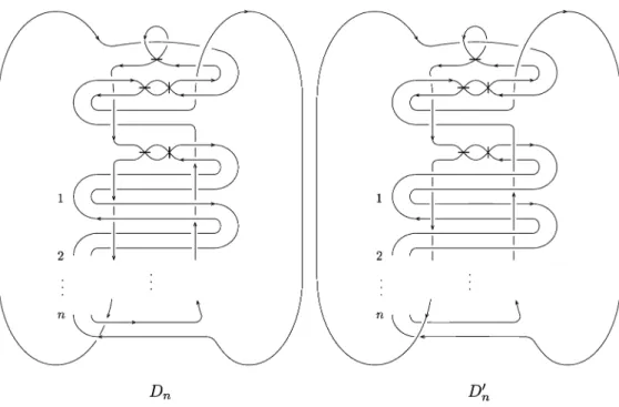
(10) 107. D_{n}'. D_{n} Figure. 10: \mathrm{H} ‐admissible marked. [8]. A.. [9]. A. Kawauchi: Three dualities. manifolds, Osaka. J. Math. 23. on. [11]. A. Kawauchi:. [12]. A. Kawauchi and S.. of. Normal. integral homology of infinite cyclic coverings of 633‐651.. theory, Birkhäuser,. cross‐section. four‐space, I;. an. immersed. 1996.. sphere‐link. in. 4‐space, Topology. Kojima: Algebraic classification of linking pairings Annalen, 253 (1980), 29‐42.. on. 3‐. Mathematische. A. Kawauchi and J. Kim: Immersed 2‐knots with essential. singularity, preprint,. 2017.. Kurlin, All 2‐dimensional links in 4‐space live inside a universal polyhedron, Algebr. Geom. Topol. 8 (2008), no. 3, 1223‐1247.. C. Kearton and V. 3‐dimensional J.. Kim,. Y.. Joung and S. Y. Lee, On the Alexander biquandles of oriented surface‐ graph diagrams, J. Knot Theory Ramifications 23(7) (2014), Article. links via marked. ID:1460007,. [16]. a. in. D_{n}'. Appl. (to appear). manifolds,. [15]. On. the. (1986),. A. Kawauchi: A survey of knot. [14]. and. Kawauchi, T. Shibuya, S. Suzuki, Descriptions on surfaces forms, Math. Sem. Notes Kobe Univ. 10 (1982), 75‐125.. [10]. [13]. graph diagrams D_{n}. 26 pp.. J. Levine: Knot modules.. I,. Trans. Amer. Math. Soc. 229. (1977),. 1‐50..

(11) 108. [17]. Surface‐links with square‐type ch‐graphs, Proceedings of the First Joint Japan‐Mexico Meeting in Topology (Morelia, 1999), Topology Appl. 121 (2002),. M. Soma:. 231‐246.. [18] [19]. Swenton, On a calculus for 2‐knots Ramifications 10 (2001), 1133‐1141.. F. J.. Yoshikawa, An. K.. and surfaces in. enumeration of surfaces in. 497‐522.. OCAMI Osaka. City University. Osaka 558‐8585. JAPAN \mathrm{E} ‐mail address:. [email protected]‐cu.ac.jp. Knot. Theory. J. Math. 31. (1994),. 4‐space, J.. four‐space, Osaka.

(12)