Bifurcation
diagram for interior single-peak solutions
in
a
Neumann
problem
for
$u”+\lambda(-u+u^{p})=0$
with
$p\in \mathbb{R}$
and
$p>1^{*}$Kazuyuki Yagasaki
$\dagger$Department of Mathematics,
Hiroshima University
1
Introduction
Let $p\in \mathbb{R}$ and $p>1$ . We study a Neumann problem for a second-order differential
equation,
$u”+\lambda(-u+u^{p})=0$ in $(-1,1)$, $u’(\pm 1)=0$, (1)
where $\lambda>0$ is
a
constant and representsa
control parameter. Eq. (1) hasa
trivialsolution $u=1.$
We often encounter (1) in several situations. As
an
example,we
consider theKeller-Segel model for chemotaxis aggregation,
$u_{t}=D_{1}u_{xx}-c(u(\log v)_{x})_{x},$ $v_{t}=D_{2}v_{xx}-av-bu$ in $(-1,1)$,
(2)
$u_{x},$$v_{x}=0$ at $x=\pm 1,$
where $D_{1},$ $D_{2},$$a,$$b,$$c$
are
constants. The stationary problem for (2) becomes$D_{2}v_{xx}-av-b\mu v^{c/D_{1}}=0, v_{x}=0atx=\pm 1$ (3)
since $D_{1}u_{x}-cu(\log v)_{x}=0$ bythe first equation, so that $u=\mu v^{c/D_{1}}$ for
some
constant$\mu.$Eq. (3) istransformed to (1). Another exampleis related to the
Gierer-Meinhardt
modelfor biological pattern formations,
$u_{t}=D_{1}u_{xx}- \mu_{1}u+\rho_{1}(c_{1}\frac{u^{p_{1}}}{v^{q_{1}}}+\rho_{0})$ , $v_{t}=D_{2}v_{xx}- \mu_{2}v+\rho_{2}c_{2}\frac{u^{p_{2}}}{v^{q_{2}}}$ in $(-1,1)$,
(4)
$u_{x},$$v_{x}=0$ at $x=\pm 1,$
’This work was partially supported by the Japan Society for the Promotion of Science, Grant-in-Aid
for Scientific Research (C) (SubjectNos. 21540124 and 22540180). Some part of this article contains a
collaboration withYasuhito Miyamoto at theUniversity of Tokyo.
$\dagger$
Present address: DepartmentofApplied Mathematics andPhysics, Kyoto University, Yoshida
$\frac{\pi^{2}}{p-1}$
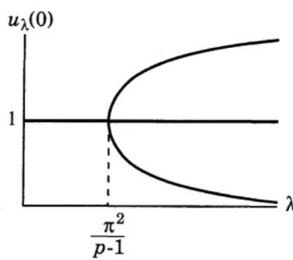
Figure 1: Bifurcation diagram for the Neumann problem (1)
where $D_{i},p_{i},$$q_{i},$$\mu_{i},$$\rho_{i},$ $i=1$,2,
are constants. As
$D_{2}arrow\infty,$ $v_{xx}arrow 0$so
that $v_{x}arrow 0$ by theboundary conditions. Hence, in this limit,
we
have$\int_{0}^{1}(\mu_{2}v-\rho_{2}c_{2}\frac{u^{p_{2}}}{v^{q_{2}}})dx=0,$
so
that$v^{q_{2}+1}= \frac{\rho_{2}c_{2}}{\mu_{2}}\int_{0}^{1}u^{p_{2}}dx$
by regarding?1 as a constant. Thus, for the stationary problem for (4), we obtain the shadow system,
$D_{1}u_{xx}- \mu_{1}u+\rho_{1}(c_{1}\frac{u^{p_{1}}}{\xi^{q_{1}}}+\rho_{0})=0, u_{x}=0atx=\pm 1,$
which is transformed to (1) like (3).
The following theorem for (1)
was
proved for $p\in \mathbb{Z}$ in [1] and for$p\in \mathbb{R}\backslash \mathbb{Z}$ in [2].Theorem 1. The branch
of
interior single-peak solutions emanatesfrom
$(\lambda, u)=(\pi^{2}/(p-$1), 1) and the
bifurcation
is a supercriticalpitchforkone.
The branch is a graphof
$\lambda$and
unbounded in $\lambda$. Moreover, each solution
of
the branch is non-degenerate and the Morseindex is two.
Here the Morse index is the number of strictly positive eigenvalues for the associated linear problem
$\phi"+\lambda(-1+pu_{\lambda}(y)^{p-1})\phi=\mu\phi$ in $(-1,1)$, $\phi’(\pm 1)=0,$
where $u_{\lambda}(y)$ represents a solution of the Neumann problem. The last part
of Theorem 1
is obvious from the other partssince $\mu=\lambda(p-1)$,$\lambda(p-1)-\frac{1}{4}\pi^{2}$
are
positive eigenvaluesof the linear problem for the trivial solution $u=1$ when $\lambda<\pi^{2}/(p-1)$, and so is $\mu=\lambda(p-1)-\pi^{2}$ when $\lambda>\pi^{2}/(p-1)$. The bifurcation diagram stated in Theorem 1 is
sketched in Fig. 1. The upperbranch represents interior single-peak solutions. In the rest of this article
we
outline the proofof Theorem 1.Figure 2: One-parameter family of periodic orbits in (5)
2
Monotonicity
of the
period
functions
Using
a
transformation $x\mapsto x/\sqrt{\lambda}$,we
rewrite (1)as
$u”-u+u^{p}=0$. (5)
For any $u_{1}\in(0,1)$ Eq. (5) has
a
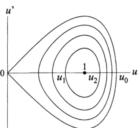
periodic solution satisfying $(u(O), u’(O))=(u_{1},0)$. Let$T(u_{1})$ denote its period and let $u_{2}\in(1, u_{0})$ satisfy $F(u_{2})=F(u_{1})$, where
$F(u)=- \frac{1}{2}u^{2}+\frac{1}{p+1}u^{p+1}+\frac{p-1}{2(p+1)}, u_{0}=p-\sqrt[1]{\frac{1}{2}(p+1)}.$
Then we have $(u( \frac{1}{2}T(u_{1})), u’(\frac{1}{2}T(u_{1})))=(u_{2},0)$
.
Note that$F(u_{0})=F(0)= \frac{p-1}{2(p+1)}.$
As shown in Fig. 2, there exists
a
one-parameter family of periodic orbits in (5).The periodic solution $u(x)$ in (5) gives an interiorsingle-peak solution in the Neumann
problem (1) when $\frac{1}{2}T(u_{1})=2\sqrt{\lambda}$. Hence, except the last part, Theorem 1 immediately
follows from the following theorem.
Theorem 2. The period
function
$T(u_{1})$ in (5) is strictly decreasingon
$(0,1)$.To prove this theorem, we use a result of Chicone [3]. We first recall his result. Let
$\xi_{1}<0<\xi_{2}$ and let $I=(\xi_{1}, \xi_{2})\subset \mathbb{R}$. Suppose that $V$ : $Iarrow \mathbb{R}$ is a $C^{3}$ function satisfying
$V(\xi_{1})=V(\xi_{2})$ and having a minimum $V(O)=0$ as its only extremum. Consider
second-order differential equations of the form
$\xi"+\frac{dV}{d\xi}(\xi)=0$
.
(6)Eq. (6) has the trivial solution $\xi=0$, and any solution $\xi=\xi(t)$ of (6) with $\xi(0)\in I\backslash \{O\}$
and $\xi’(0)=0$ is periodic. Let $T(h)$ be its period with $h=V(\xi(0))$, and define a function
$\varphi(\xi)$
as
$\varphi(\xi)=\frac{V(\xi)}{V’(\xi)^{2}}$. (7)
Proposition 3 (Chicone [3]). Suppose that
$\varphi"(\xi)\geq 0 for\xi\in I\backslash \{O\}$ (8)
and the inequality holds in
a
punctured neighborhoodof
$\xi=$ O. Then $T(h)$ is strictlyincreasing on $(0, h_{0})$, where $h_{0}=V(\xi_{1})(=V(\xi_{2}))$.
3
Proof of Theorem 2
Using a transformation $u=\xi+1$
we
rewrite (5)as
the form of (6) with $\xi_{1}=-1,$$\xi_{2}=u_{0}-1>0$ and $V(\xi)=F(\xi+1)$. We compute (7)
as
$\varphi"(\xi)=\frac{(p-1)g(\xi+1)}{(p+1)(\xi+1)^{4}((\xi+1)^{p-1}-1)^{4}}$, (9)
where
$g(u)=pu^{3p-1}-(2p^{2}-3p+3)u^{2p}+p(2p+1)u^{2p-2}$
$-p(p-2)u^{p+1}+p(p-7)u^{p-1}+3.$
We begin with the
case
of$p\in \mathbb{Z}$ with $p>1$. We easilysee
that the function $g(u)$ isdivisible by $(u-1)^{4}$ and define $a$ $(3p-5)$-th order polynomial $\overline{9}(u)=g(u)/(u-1)^{4}$. After
some
highly nontrivial computations,we
prove the following (see [1] for the proof). Lemma 4. Allcoefficients
of
$g(u)$are
positive.From Lemma4 and (9) we see that
$\varphi"(u-1)=\frac{(p-1)\overline{g}(u)}{(p+1)u^{4}(\sum_{j=0}^{p-2}u^{j})^{4}}>0$ for
$u\in(0, u_{0})$,
i.e., condition (8) holds.
We next
assume
that$p\in \mathbb{Q}\backslash \mathbb{Z}$with$p>1$. Let$p=m/n>1$ , where$m,$$n$
are
relativelyprime integers and $n\geq 2$. We set $v=u^{1/n},$
$k=m-n>0$
and $\psi(v)=n^{2}g(v^{n})$ to have$\psi(c))=n(n+k)v^{2n+3k}-(2k^{2}+kn+2n^{2})v^{2n+2k}+(n-k)(n+k)v^{2n+k}$
$+(n+k)(3n+2k)v^{2k}-(n+k)(6n-k)v^{k}+3n^{2}$
We easily
see
that the polynomial $\psi(v)$ is factorizedas
$\psi(v)=(v-1)^{4}\overline{\psi}(v)$, where $\overline{\psi}(v)$is$a$ $(2n+3k-4)$-th
order
polynomial. We also provethe following (see [2] for the proof).Lemma 5. All
coeficients of
$\overline{\psi}(v)$ are positive.From Lemma 5 and (9) we
see
that$\varphi"(\tau)^{n}-1)=\frac{(p-1)\overline{\psi}(v)}{(p+1)n^{2}v^{4n}(\sum_{j=0}^{k-1}v^{j})^{4}}>0$ for $v\in(0, \sqrt[n]{u_{0}})$.
i.e., condition (8) holds again.
We turnto the caseof$p\in \mathbb{R}\backslash \mathbb{Q}$with$p>1$. Take
a
sequence $\{p_{j}\}_{j=0}^{\infty}$ such that$p_{j}\in \mathbb{Q}$and $\lim_{jarrow\infty}p_{j}=p$. We easily see that condition (8) holds for $p\in \mathbb{R}\backslash \mathbb{Q}$ since it does for
References
[1] Y. Miyamoto aIld K. Yagasaki, Monotonicity of the first eigenvalue and the global
bifurcationdiagram for thebranch ofinterior peaksolutions, J.
Differential
Equations,254
(2013),342-367.
[2] K. Yagasaki, Monotonicity of the period function for $u”-u+u^{p}=0$ with p $\in \mathbb{R}$ and
p $>$ 1, J.
Differential
Equations, 255 (2013),1988-2001.
[3] C. Chicone, The monotonicity of the period function for planar Hamiltonian vector