AN EXPLICIT DESCRIPTION OF THE RADIATION FIELD IN $3+1$-DIMENSIONS (Spectral and Scattering Theory and Related Topics)

全文

(1)40. 数理解析研究所講究録第2023巻 2017年 40-49. AN EXPLICIT DESCRIPTION OF THE RADIATION FIELD IN. 3+1 ‐DIMENSIONS DEAN BASKIN. ABSTRACT. In previous work with A. Vasy and J. Wunsch, the author established an asymptotic expansion for the radiation field on asymptotically Minkowski spacetimes and showed that the exponents seen in the expansion are given by the poles of a meromorphic. family of operators on the spacetimes boundary at infinity. This note provides an explicit accounting of these poles when the spacetime is 3+1 ‐dimensional Minkowski space. We conclude by stating the resonant states for the first few resonances and then posing a combinatorial problem.. 1. INTRODUCTION. For. a. forward solution. u. of the inhomogeneous. equation. wave. \square u=f\in C_{\mathrm{c} ^{\infty}(\mathbb{R}^{3}\times \mathbb{R}). on. Minkowski space,. ,. (or, equivalently, a solution u of the homogeneous wave equation with compactly sup‐ ported initial data), the Friedlander radiation field of u encodes the behavior of u near null infinity. With A. Vasy and J. Wunsch [1, 2], the author established an asymptotic expansion of the radiation field on a class of asymptotically Minkowski spacetimes and showed that the exponents of the expansion were given by the poles of a meromorphic family of operators (called P_{ $\sigma$}^{-1} in those papers) on the boundary at infinity. The pur‐ pose of this note is to identify explicitly these poles in the setting of (3+1) ‐dimensional Minkowski space. In particular, we prove the following theorem: poles of P_{ $\sigma$}^{-1} are simple and located at - $\iota$(k+1) for k=0 1, 2, of polar part of P_{ $\sigma$}^{-1} at $\sigma$=- $\iota$(k+1) is \displaystyle \sum_{J^{=0}}^{k}\dim(E_{j})=(k+1)^{2} where E_{J} the eigenspace of \triangle_{\mathrm{S}^{2} with eigenvalue j.. Theorem 1. The The rank is. .. ,. the. .. .. .. ,. The rest of the introduction is devoted to. Suppose. that. u. is the solution of the. forward solution of the. inhomogeneous. explaining and motivating Theorem 1. homogeneous wave equation (or, equivalently,. wave. equation). o. \mathrm{a}. \mathrm{n}^{\mathrm{t} 3+1 ‐dimensional Minkowski. space:. \square u=\partial_{t}^{2}-\triangle u=0 \mathrm{i}\mathrm{n}\mathbb{R}\times \mathbb{R}^{3} (u, \partial_{t}u)|_{t=0}=( $\phi,\ \psi$)\in C_{c}^{\infty}(\mathbb{R}^{3})\times C_{c}^{\infty}(\mathbb{R}^{3}) introduce polar coordinates (r, $\omega$) in the spatial variables parameter s=t-r and define an auxiliary function We. now. v(r, s, $\omega$)=r^{-1}u(s+r,r $\omega$) Date: 11. April. The author is. as. well. as a. $\iota$. lapse. .. 2016.. grateful. to. Semyon Dyatlov for. an. observation. conducted with the support of NSF grant DMS‐1500646.. leading. to this note. This research was.

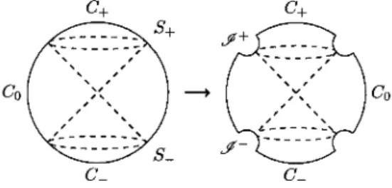
(2) 41 DEAN BASKIN. Friedlander. [3]. observed that the function. v. $\rho$=0 The Friedlander radiation field of. to. .. is smooth in u. is then. $\rho$=r^{-1}. and. so can. be extended. given by. \displaystyle \mathcal{R}_{+}[u](s, $\omega$)=\lim_{r\rightar ow\infty}\partial_{s}v(r, s, $\omega$). .. In Minkowski spaces (and other static spacetimes), the radiation field has a number of desirable properties: Not only is it a unitary translation representation of the wave group,. also be. thought. of. it. can. in. \mathbb{R}\times \mathbb{R}^{3} if the initial data. of. as. ,. generalizing are. $\psi$.). (0, $\psi$). ,. the Radon transform of the initial data.. then the radiation field is. (Indeed,. just the Radon transform. previous work [1, 2], the author and collaborators showed that the radiation field ad‐ asymptotic expansion for suitably nice data. Indeed, on a class of asymptotically Minkowski spacetimes, the radiation field exists and admits an asymptotic expansion in powers of s^{-1} The exponents seen arise as the poles of a meromorphic family of Fredholm operators, denoted P_{ $\sigma$}^{-1} on the boundary at infinity In. mits. an. .. We let M denote the radial. compactification of Minkowski space with a defining function boundary. In other words, we can consider \mathbb{R}\times \mathbb{R}^{3} as the interior of a compact manifold with boundary via the coordinate change $\rho$ for the. t=\displaystyle\frac{1}{$\rho$}\cos$\theta$, x=\displayst le\frac{1} $\rho$} \omega$ sine,. $\omega$_{j}\in \mathrm{S}^{2} and $\theta$\in \mathrm{S}^{1} We denote by c_{\pm} (depending on the sign of t) the regions of boundary sphere X\cong \mathrm{S}^{3} corresponding to where |t|\gg|x| while we denote by C_{0} the region of X where |t|\ll|x| These regions of X naturally inherit conformal families of metrics; on Minkowski space, c_{\pm} are naturally conformal to \mathbb{H}^{3} and C_{0} is naturally where. .. the. ,. .. conformal to 2+1 ‐dimensional de Sitter space. It is the region where |t|\sim|x| that is of the most interest; we denote these regions by s_{\pm} depending on the sign of t By blowing up (in the algebro‐geometric sense) the .. submanifolds s_{\pm} in M we obtain a manifold with corners that has two new boundary faces, denoted \mathcal{I}^{\pm} and corresponding to past and future null infinity. Figure 1 provides a ,. schematic view of this of. u. to. \mathcal{I}^{+}.. blow‐up.. The radiation field. \mathcal{R}_{+}[u]. is then the rescaled restriction. FIGURE 1. A schematic view of the. along \mathcal{I}^{+} towards C_{+} c_{\pm} are collapsed to i\pm .. Conjugating yields a family. \square. by. $\rho$ ,. blow‐up. The lapse function s increases typical Penrose diagram of Minkowski space, and C_{0} is collapsed to i_{0}.. In the. multiplying by $\rho$^{-2} and then taking the on the boundary sphere X\cong \mathrm{S}^{3}. of operators P_{ $\sigma$}. ,. .. Mellin transform in $\rho$ This has the effect of.

(3) 42 THE RADIATION FIELD IN 3+1 ‐DIMENSIONS. $\rho$\partial_{ $\rho$} in $\rho$^{-3}\square $\rho$ by $\iota \sigma$ Although P_{ $\sigma$} is semiclassically hyperbolic hyperbolic), on c_{\pm} it is classically elliptic (indeed, it can be conjugated spectral family for the Laplacian on hyperbolic space). On C_{0}, P_{ $\sigma$} is hyperbolic. replacing. all factors of. (because. \square is. to the. and. can. be. conjugated. .. to. a. Klein‐Gordon equation. on. de Sitter space, while at s_{\pm} it is. degenerate. The Hamilton vector field of the. symbol of P_{ $\sigma$} is radial at the conormal bundle of s_{\pm} techniques dating back to Melrose [5] and refined by Vasy [6] provide a blueprint for establishing propagation estimates there. The operator family P_{ $\sigma$} is not Fredholm on standard Sobolev spaces, but it is when considered on variable‐order Sobolev spaces whose regularity lies below some threshold at S_{-} (depending on the imaginary part of $\sigma$ ) and is larger than a similar threshold at s_{+} (again, depending on the imaginary part of $\sigma$ ). As P_{ $\sigma$} is then invertible on these spaces for very large {\rm Im} $\sigma$ we may invert to obtain a meromorphic family of Fredholm operators P_{ $\sigma$}^{-1}. Because all light rays in Minkowski space escape to infinity, P_{ $\sigma$}^{-1} has only finitely many poles in any horizontal strip in \mathb {C} The main result of both previous papers [1, 2] is that and. so. ,. .. the radiation field for are. these poles, which. operator. at. a. forward solution has. are. identified. as. the. an. asymptotic expansion whose exponents of the asymptotically hyperbolic. resonances. C_{+}.. For 3+1 ‐dimensional Minkowski space, however, this asymptotically hyperbolic op‐ erator is the spectral family of the Laplacian on \mathbb{H}^{3} , which has no resonances. In this case, the. than. resonant.states associated. \overline{C_{+} ).. to the. poles. of. P_{ $\sigma$}^{-1}. Theorem 1 describes the locations of these. supported in s_{+} (rather poles and the dimension of the. must be. corresponding nullspace of P_{ $\sigma$}. The proof of Theorem 1 proceeds in several steps. We first recall from [1] that any resonant state must be supported at the intersection of the light cones and the boundary at infinity because odd‐dimensional hyperbolic space has no resonances. This reduces the problem of finding the poles of P_{ $\sigma$}^{-1} (and the corresponding resonant states) to under‐ standing when P_{ $\sigma$} has nullspace consisting of a distribution of the form. \displayst le\sum_{k=0}^{M}a_{k}$\delta$^{(k)}(v)\otimes$\phi$_{$\lambda$},. where. $\phi$_{$\lambda$} is a spherical harmonic with eigenvalue $\lambda$ This immediately implies that the poles of P_{ $\sigma$}^{-1} are contained in the negative imaginary integers and reduces the problem of finding the null spaces of an explicit family of matrices. For $\sigma$=- $\iota$(M+1) P_{ $\sigma$} preserves the family of such distributions and so the problem of finding the null space of P_{ $\sigma$} reduces to a linear algebra problem. We write down the matrix representing P_{ $\sigma$} and compute its determinant explicitly. This shows that the matrix has one‐dimensional null space M and hence that P_{- $\iota$(M+1)} has null space precisely when $\lambda$=k(k+1) for k=0 1, .. ,. ,. .. .. .. ,. of dimension. where. E_{k} is the. space of. \displaystyle\sum_{k=0}^{M}\dim(E_{k}). ,. spherical harmonics with eigenvalue k(k+1) the elements of the null space explicitly is sufficiently compli‐ cated that we were unable to solve it here by purely combinatorial means. It is perhaps surprising how difficult it is to find an explicit expression for elements of the nullspace of P_{- $\iota$(k+1)} However, given the connection of the radiation field with the Radon trans‐ form, such an expression would provide an explicit formula for the Radon transform in. Unfortunately, finding. .. ..

(4) 43 DEAN BASKIN. terms of spherical harmonics. Such formulas representation‐theoretic underpinnings).. In Section 2. we. describe. some. space, and then in Section 3. We also introduce. following. a. exist but. are. similarly complicated (and have. of the geometry of the radial compactification of Minkowski define the operator P_{ $\sigma$} and recall some of its properties.. we. convenient coordinate. system that simplifies the linear algebra. section. Section 4 recasts the. of. in the. problem describing poles corresponding algebra and finishes the proof of Theorem 1. Included exact form of the resonant states corresponding to the first few poles Section 5 we conclude by appealing for a combinatorial expression for the. and. resonant states in terms of linear. in Section 4 is the. of. P_{ $\sigma$}^{-1} Finally, .. in. the elements of the null space of P_{ $\sigma$} in this context.. 2. GEOMETRY. The radiation field is the rescaled restriction of null. infinity.. In this section. this statement is We. a. natural. begin by introducing. we. describe. a. solution. u. of the. wave. compactification of Minkowski. a. equation. space. on. to. which. one.. coordinates. on. Minkowski space given. by. t=\displaystyle\frac{1}{$\rho$}\cos$\theta$ x=\displaystyle\frac{1}{$\rho$} \omega$_{j}\sin$\theta$ where. We. $\omega$_{J}\in \mathrm{S}^{2}. .. In terms of these. coordinates, the. metric. on. Minkowski space is given. by. g:=-dt^{2}+\displaystyle\sum_{j=1}^{3}dx_{j}^{2}=-\cos2$\theta$\frac{d$\rho$^{2}{$\rho$^{4}-4\sin$\theta$\cos$\theta$\frac{d$\theta$}{$\rho$}\frac{d$\rho$}{$\rho$^{2}+\cos2$\theta$\frac{d$\theta$^{2}{$\rho$^{2}+\sin^{2}$\theta$\frac{dw^{2}{$\rho$^{2} now. replace the coordinate $\theta$ by v=\cos 2 $\theta$. to obtain. g=-v\displaystyle\frac{d$\rho$^{2} {$\rho$^{4} +\frac{dv}{$\rho$}\frac{d$\rho$}{$\rho$^{2} +\frac{v}{4(1-v^{2}) \frac{dv^{2} {$\rho$^{2} +\frac{1-v}{2}\frac{d$\omega$^{2} {$\rho$^{2} The inverse metric. (in. coordinates. ( $\rho$, v, $\omega$) ). is then. given by. g^{-1}\displayst le\rightarow(21^{-v$\rho$^{4}-v^{2})$\rho$^{3}04v(1-v^{2})$\rho$^{2} (1-v^{2})$\rho$^{3}0\frac{2$\rho$^{2}{1-v}h^{-1}0 ). where h is the standard This radial. (round). metric. on. ,. \mathrm{S}^{2}.. compactification of Minkowski space has two distinguished submanifolds where $\rho$=0 and v=0, \mathrm{w}\mathrm{h}\mathrm{i}\mathrm{c}\grave{\mathrm{h} we call s_{\pm}(S_{\pm} are distinguished by the sign of t-S_{+} is the set in the future where $\rho$=0 and v=0 while S_{-} is the corresponding set in the past). ,. 3. THE. The central. object of study. OPERATORS. is the operator L ,. given by. L=$\rho$^{-3}\square _{g} $\rho$. Here the conjugation by $\rho$ should be thought of as accounting for the standard decay for solutions of the wave equation, while the prefactor of $\rho$^{-2} turns a scattering operator in the sense of Melrose [5] into a b‐‐operator [4]..

(5) 44 THE RADIATION FIELD IN 3+1 ‐DIMENSIONS. We record here the. precise form of L :. L=v( $\rho$\partial_{ $\rho$})^{2}+(2+4v) $\rho$\partial_{ $\rho$}-4(1-v^{2}) $\rho$\partial_{ $\rho$}\partial_{v}. -4v(1-v^{2})\displaystyle \partial_{v}^{2}-4(1-v-3v^{2})\partial_{v}-\frac{2}{1-v}\triangle_{w}+(2+3v) \hat{N}(L)( $\sigma$). The operator P_{ $\sigma$} is the reduced normal operator which effectively , $\rho$\partial_{ $\rho$} by $\iota \sigma$ and is obtained by conjugating L by the Mellin transform in $\rho$ :. replaces. P_{ $\sigma$}=-v$\sigma$^{2}+(2+4v) $\iota \sigma$-4 $\iota \sigma$(1-v^{2})\partial_{v}. -4v(1-v^{2})\displaystyle \partial_{v}^{2}-4(1-v-3v^{2})\partial_{v}-\frac{2}{1-v}\triangle_{ $\omega$}+(2+3v) Although. the. expression above for P_{ $\sigma$} is useful for the global problem of identifying the properties of F_{ $\sigma$} for our explicit computation it is more conveniènt to work with different coordinate system valid near S_{+} For the remainder of this note, we instead. Fredholm a. ,. .. take. In these. coordinates,. $\rho$=\displaystyle \frac{1}{t+r}, v=\frac{t-r}{t+r}. we. may write. \displaystyle \square =\partial_{t}^{2}-\partial_{r}^{2}-\frac{2}{r}\partial_{r}-\frac{1}{r^{2} \triangle_{ $\omega$}. =4$\rho$^{2}[- $\rho$\displaystyle \partial_{ $\rho$}\partial_{\bul et}-\partial_{v}-v\partial_{v}^{2}+\frac{1}{1-v}( $\rho$\partial_{ $\rho$}+(1+v)\partial_{v})-\frac{1}{(1-v)^{2} $\Delta$_{ $\omega$}]. We then have. L=$\rho$^{-3}\displaystyle \square $\rho$=4[- $\rho$\partial_{ $\rho$}\partial_{v}-2\partial_{v}-v\partial_{v^{2} +\frac{1}{1-v}( $\rho$\partial_{ $\rho$}+1+(1+v)\partial_{v})-\frac{1}{(1-v)^{2} \triangle_{ $\omega$}] and. P_{ $\sigma$}=4[-( $\iota \sigma$+2)\displaystyle \partial_{v}-v\partial_{v}^{2}+\frac{ $\iota \sigma$+1}{1-v}+\frac{1+v}{1-v}\partial_{v}-\frac{1}{(1-v)^{2} \triangle_{ $\omega$}].. We may then. homogeneity:. multiply P_{ $\sigma$} by (1-v)^{2}/4. and group the terms with the. same. degree. of. \displaystyle \frac{(1-v)^{2} {4}P_{ $\sigma$}=[-( $\iota \sigma$+1)\partial_{v}-v\partial_{v}^{2}]. +[2( $\iota \sigma$+2)v\partial_{v}+2v^{2}\partial_{v}^{2}+( $\iota \sigma$+1)- $\Delta \omega$] +[-( $\iota \sigma$+3)v^{2}\partial_{v}-v^{3}\partial_{v}^{2}-( $\iota \sigma$+1)v] 4. THE POLES OF. At each. pole. of. P_{ $\sigma$}^{-1}. P_{ $\sigma$}^{-1}. can be identified with an operator whose image is self‐adjoint, the residue operators do not project onto these states, but we abuse terminology by calling them resonant states anyway. We know from the results of [1] that if f is supported away from \overline{C_{-} then P_{ $\sigma$}^{-1}f is supported in \overline{C_{+} Moreover, if P_{ $\sigma$}^{-1}f is not supported in s_{+} then the pole (and corresponding state) can be identified with a resonance of a Laplace‐like operator on C_{+} In n+1 ‐dimensional Minkowski space, this operator is the Laplacian on \mathbb{H}^{n}. \mathrm{a}. (resonant state. ,. the residue. As P_{ $\sigma$} is not. ,. .. ,. ..

(6) 45 DEAN BASKIN. Because \mathbb{H}^{3} has. no. we. resonances,. can. conclude that all resonant states of. 3+1‐dimensional Minkowski space must be therefore be sums of the following form:. \displayst le\sum_{k=0}^{M}$\alpha$_{k}$\delta$^{(k)}(v)\otimes$\phi$_{$\lambda$}($\omega$). (1) where. $\phi$_{$\lambda$}. supported. is. a. spherical harmonic with eigenvalue $\lambda$. section, we prove Theorem 1 in. In the rest of this. action of. P_{ $\sigma$}. such. on. a. sum, which shows that. P_{ $\sigma$} has. in. s_{+}. .. P_{ $\sigma$}^{-1}. on. The resonant states must. ,. several no. steps. We first compute the. null space unless. \displaystyle \frac{(1-v)^{2} {4}P_{ $\sigma$}. $\sigma$=- $\iota$(M+1). for M=0 1, For such a $\sigma$ we then interpret (which has the same null space as P_{ $\sigma$} when acting on such distributions) as a family of matrices depending on $\lambda$. We compute this determinant and show that the matrix has a 1‐dimensional null space .. ,. exactly. when. We. now. the. .. .. ,. $\lambda$=k(k+1). of the space of Theorem 1. on. .. spherical. for k=0 , 1,. harmonics with. record the action of. following. \displaystyle \frac{(1-v)^{2} {4}P_{ $\sigma$}. .. .. .. ,. M. Appealing. .. to the well‐known dimension. eigenvalue k(k+1) then completes the proof of on. distributions of the form above. well‐known fact:1. We then have the. (1).. We. rely. v^{r}$\delta$^{k}(v)=\displaystyle \frac{k!}{(k-r)!}$\delta$^{(k-r)}(v). following:. \displaystyle \frac{(1-v)^{2} {4}P_{ $\sigma$}($\delta$^{(k)}(v)\otimes$\phi$_{ $\lambda$}( $\omega$) =[(- $\iota \sigma$+1)+(k+2)]$\delta$^{(k+1)}\otimes$\phi$_{ $\lambda$}. +[-( $\iota \sigma$+1)(2k+1)+2(k+1)^{2}+ $\lambda$]$\delta$^{(k)}\otimes$\phi$_{ $\lambda$} +[-( $\iota \sigma$+1)k^{2}+k^{2}(k+1)]$\delta$^{(k-1)}\otimes$\phi$_{ $\lambda$}. particular, for. In. must vanish and. apply P_{ $\sigma$}. to such. a sum so a. (2). of the form. (1). to lie in the null space of. M+1- $\iota \sigma$=0 i.e., $\iota \sigma$=M+1. P_{ $\sigma$} the leading ,. We may then take sum, and rearrange the terms to find the following: ,. .. term. $\sigma$=- $\iota$(M+1). ,. \displaystyle \frac{(1-v)^{2} {4}P_{- $\iota$(M+1)}(\sum_{k=0}^{M}$\alpha$_{k}$\delta$^{(k)}(v)\otimes$\phi$_{ $\lambda$}( $\omega$) =\sum_{k=0}^{M}[(k-1-M)$\alpha$_{k-1}. +( $\lambda$+2k^{2}-M(2k+1))$\alpha$_{k}. We have. +(k+1)^{2}(M-k)$\alpha$_{k+1}]$\delta$^{(k)}(v)\otimes$\phi$_{ $\lambda$}( $\omega$). reduced the. problem to finding a vector of coefficients $\alpha$_{k} so that the sum (2) vanishes. This is equivalent to finding the null space of a matrix $\lambda$ I-A_{M} where A_{M} is the tridiagonal (M+1)\times(M+1) ‐matrix with the following entries: now. ,. a_{k,k}=(M-k)(2k+1)+k. a_{k-1,k}=-k^{2}(M+1-k) a_{k,k-1}=M+1-k Here all indices. This. formula is. (k a. and k-1 ) should be. interpreted. priori valid only for r\leq k but if. denominator is infinite for r>k and. ,. so. the. we. right‐hand side. as. taking the values. 0,. 1,. .. .. .. ,. M.. interpret (k-r)!= $\Gamma$(k-r+1) then the ,. is. zero. there..

(7) 46 THE RADIATION FIELD IN 3+1 ‐DIMENSIONS. The rest of the. proof of. Theorem 1 then follows from the. following proposition:. Proposition 2. The matrix A_{M} has simple eigenvalues k(k+1) for k=0 1, particular, we have that ,. \det( $\lambda$ I-A_{M})=p_{M}( $\lambda$). .. .. .. ,. M. In. ,. where. Proposition. 2 follows. p_{k}($\lambda$)=\displaystyle\prod_{J^{=0} ^{k}($\lambda$-j( +1 immediately by taking. k=M in the. following. lemma:. Lemma 3. Let. of 0,. d_{k} be the determinant of the (k+1)\times(k+1) ‐minor of $\lambda$ I-A_{M} consisting columns and rows of the matrix (i.e_{f} the columns and rows labeled k+1 first. the. 1,. .. .. .. ,. k) If p_{k}( $\lambda$) .. as. in. Proposition 2, then. d_{k}=\displaystyle \sum_{l=0}^{k+1}c_{k.\el }(\prod_{j=1}^{p}(M-k+P-j) p_{k-\el }( $\lambda$). where. and. is. interpret p_{-1}( $\lambda$)=1.. we. ,. c_{k,l}=\displaystyle \frac{(-1)^{\el } {\el !}(\frac{(k+1)!}{(k+1-l)!})^{2}. Observe that all terms containing p_{k-\ell}( $\lambda$) with \ell\geq 1 in the expression for d_{k} in Lemma 3 multiplied by a factor (M-k) and hence vanish when k=M leaving only the term. are. ,. c_{M,\mathrm{f}\} p_{M}( $\lambda$)=p_{M}( $\lambda$) Proof of Lemma. .. 3. The matrix A_{M} is. tridiagonal,. so. d_{k}. can. be. computed recursively:. d_{k}=( $\lambda$-a_{k,k})d_{k-1}+a_{k,k-1}a_{k-1,k}d_{k-2}. We therefore. proceed by induction, interpreting d_{-1}=1 so that the lemma holds for k=-1 In particular, we have c_{-1,0}=1 and c_{-1,\ell}=0 for \ell\geq 1. In computing below, we use the following relationship between the p_{k} : .. $\lambda$ p_{k-1-l}( $\lambda$)=p_{k-\ell}( $\lambda$)+(k-\ell)(k-l+1)p_{k-1-l}( $\lambda$) We. now. compute the. two terms in the recursive. expression for d_{k}. .. We first have the. following:. ( $\lambda$-a_{k,k})d_{k-1}. =( $\lambda$-(M-k)(2k+1)-k) \displaystyle \sum_{l=0}^{k}c_{k-1,\el }(\prod_{j=1}^{\el }(M-k+1+\el -j) p_{k-1-\el }( $\lambda$) =\displaystyle \sum_{l=0}^{k}c_{k-1,l}(\prod_{j=0}^{\el -1}(M-k+P-j) p_{k-\el }( $\lambda$) +\displaystyle \sum_{\ell=1}^{k+1}c_{k-1,\ell-1}[(k-\ell+1)(k-\ell+2)-(M-k)(2k+1)-k].. (_{J}\displaystyle \prod_{=1}^{l-1}(M-k+\el -j) p_{k-p}( $\lambda$).

(8) 47 DEAN BASKIN. The second term is. given by. a_{k,k-1}a_{k-1,k}d_{k-2}=-\displaystyle \sum_{\el =2}^{k+1}c_{k-2,\el -2}(M+1-k)^{2}k^{2}(\prod_{j=1}^{\el -1}(M-k+\el -j) p_{k-l}( $\lambda$). Adding that. the two terms and equating coefficients with the desired expression for d_{k}. ,. we. find. (M-k)c_{k,l}=(M-k+l)c_{k-1,\ell} +[(k-\ell+1)(k-P+2)-(M-k)(2k+1)-k]c_{k-1,\ell-1}. -k^{2}(M-k+1)c_{k-2,\ell-2}. We rewrite this. equation suggestively:. (M-k)c_{k,\ell}=(M-k)(c_{k-1,\ell}-(2k+1)c_{k-1,l-1}-k^{2}c_{k-2,l-2}). (3). +Pc_{k-1,\ell}+((k-\ell+1)(k-P+2)-k)c_{k-1,l-1}-k^{2}c_{k-2,l-2}. To prove the lemma, it therefore suffices to show that c_{k,\ell} is an integer. We prove this by induction. We have already seen that c_{-1,0}=1 and c_{-1,\ell}=0 for \ell\geq 1 By the. fact. .. induction. for all. hypothesis,. (k',P')<(k,P). ,. we assume. where. that. c_{k',\el '}=\displaystyle \frac{(-1)^{\el '} {(\el )!}(\frac{(k'+1)!}{(k'+1-\el )!})^{2} we. define. (a', b')<(a, b). if either. b'<b or b'=b and a'<a. ,. We turn first to the second line of equation. (3). By. the induction. hypothesis,. \ell c_{k-1,\ell}+((k-P+1)(k-\ell+2)-k)c_{k-1,\ell-1}-k^{2}c_{k-2,l-2}. =\displaystyle \frac{(-1)^{p} {(\ell-1)!}(\frac{k!}{(k-\ell+1)!})^{2}( k-P+1)^{2}-(k-\ell+1)^{2}-(k-\ell+1)+k-(\ell-1) =0. Equation (3) and the induction hypothesis then imply. that. \mathcal{C}_{k,\ell=c_{k-1,l}-(2k+1)c_{k-1,\ell-1}-k^{2}c_{k-2},p-2}. finishing. the. =\displaystyle \frac{(-1)^{p} {\ell!}(\frac{k!}{(k-\ell+1)!})^{2}( k-\ell+1)^{2}+(2k+1)P-\ell(\ell-1) =\displaystyle \frac{(-1)^{\el } {\el !}(\frac{(k+1)!}{(k-l+1)!})^{2}. proof of the lemma.. 4.1. The first few resonant states. In this section. eigenvectors of For M=0. so. the matrix. record the first five sets of. A_{M}.. ,. we. have that. For M=1 ,. we. have that. that the eigenvectors. we. are. A_{0}=(0). ,. so. its. only eigenvalue. A_{1}=\left(\begin{ar y}{l 1&\mathrm{l}\ 1&1 \end{ar y}\right),. \mathrm{v}_{0}=\left(\begin{ar y}{l -1\ \mathrm{l} \end{ar y}\right),\mathrm{v}_{2}=\left(\begin{ar y}{l 1\ 1 \end{ar y}\right).. \square. is 0 with. eigenvector (1)..

(9) 48 THE RADIATION FIELD IN 3+1 ‐DIMENSIONS. For M=2 ,. with. we. record the matrix. A_{3}=\left(bgin{ar y}{l 3& 0&\ 3&7 8&0\ &2 7&9\ 0& 1&3 \end{ar y}\ight), \mathr{v}_0=\left(bgin{ar y}{l -6\ \ -3\ 1 \end{ar y}\ight),\mathr{v}_2=\left(bgin{ar y}{l 6\ -2\ -1\ \end{ar y}\ight),\mathr{v}_6=\left(bgin{ar y}{l -6\ -6\ 3\ 1 \end{ar y}\ight),\mathr{v}_12=\left(bgin{ar y}{l 6\ 18\ 9\ mathr{l} \end{ar y}\ight). that the eigenvectors. Finally,. so. A_{2}=\left(\begin{ar y}{l 2& 0\ 2&4 \ 0&1 2 \end{ar y}\right), \mathrm{v}_0=\left(\begin{ar y}{l 2\ -2\ \mathrm{l} \end{ar y}\right),\mathrm{v}_2=\left(\begin{ar y}{l -2\ 0\ 1 \end{ar y}\right),\mathrm{v}_6=\left(\begin{ar y}{l 2\ 4\ 1 \end{ar y}\right). eigenvectors. For M=3 ,. so. have. we. are. for M=4 the matrix is ,. A_{4}=\left(bgin{ary}l 4& 0 &\ 4&mathr{l}0&\mathr{l}2&0 \ 0&312 8&0\ &021&\mathr{l}6\ 0& 1&4 \end{ary}\ight), \mathr{v}_0=\left(bgin{ary}l 24\ - \ 12 -4\ 1 end{ary}\ight), \mathr{v}_2=\left(bgin{ary}l -24\ 1 0\ -2 \mathr{l} \endary}\ight), \mathr{v}_6=\left(bgin{ary}l 24\ 1 -\mathr{l}2\ 1\end{ary}\ight), \mathr{v}_12=\left(bgin{ary}l -24\ 8\ 0 8\ 1 end{ary}\ight), \mathr{v}_20=\left(bgin{ary}l 24\96 72\16 \mathr{l} \endary}ight) that the eigenvectors. are. 5. A. We conclude this note. COMBINATORIAL PROBLEM. by posing. problem. In principle it is possible means. Specifically, this would be achieved by explicitly finding the eigenvectors of the matrix A_{M} above. The M. computation above shows that the eigenvalues are k(k+1) for k=0 to determine the resonant states of. a. combinatorial. P_{ $\sigma$}^{-1} by purely. combinatorial. ,. Problem 4. Find. a. general expression for. The resolution of this. of P_{ $\sigma$}. problem. would. the. provide. eigenvectors of the an. .. .. .. ,. matrix. explicit formula for the. A_{M}. resonant states. Minkowski space and thus give an explicit expression for the radiation field in terms of spherical harmonics. Such a formula would then make it feasible to compute the on. radiation field. explicitly for non‐trivial examples. Moreover, given the connection between the radiation. such. a. formula should also. spherical. harmonic. recover. a. field and the Radon. transform,. formula for the Radon transform in terms of. decomposition. Existing. formulas. typically rely. on. a. the Funk‐Hecke.

(10) 49 DEAN BASKIN. formula and thus involve the. Legendre polynomials.. expression for the eigenvectors of A_{M} ought. to be. We therefore expect that the general in terms of coefficients of. expressible. Legendre polynomials. REFERENCES. [1]. [2] [3] [4]. Baskin, András Vasy, and Jared Wunsch. Asymptotics of radiation fields in asymptotically Minkowski space. Amer. J. Math., 137(5):1293‐1364, 2015. Dean Baskin, András Vasy, and Jared Wunsch. Asymptotics of scalar waves on long‐range asymptot‐ ically Minkowski spaces. Preprint, arXiv: 1602.04795, 2016. Dean. F. G. Friedlander. Radiation fields and. S..oc., 88(3):483-515. ,. hyperbolic scattering theory.. Math. Proc.. Cambridge. Philos.. 1980.. Richard B. Melrose. The. Atiyah‐Patodi‐Smger index theorem, volume 4 of Research Notes m Mathe‐ Peters, Ltd., Wellesley, MA, 1993. [5] Richard B. Melrose. Spectral and scattering theory for the Laplacian on asymptotically Euclidian spaces. In Spectral and scattering theory (Sanda, lg92), volume 161 of Lecture Notes in Pure and Appl. Math., pages 85‐130. Dekker, New York, 1994. [6] András Vasy. Microlocal analysis of asymptotically hyperbolic and Kerr‐de Sitter spaces (with an appendix by Semyon Dyatlov). Invent. Math., 194(2):381-513 2013. matics. A K. ,. DEPARTMENT. OF. MATHEMATICS, TEXAS A&M UNIVERSITY, COLLEGE STATION,. E‐mad address: [email protected]. TX 77843.

(11)