PDF Fulltext | November 2016 Browse Articles 08 01191

Article

Wind Energy Potential Assessment and Forecasting

Research Based on the Data Pre-Processing Technique

and Swarm Intelligent Optimization Algorithms

Zhilong Wang1_{, Chen Wang}2,_{* and Jie Wu}3

1 _{Department of Basic Courses, Lanzhou Polytechnic College, Lanzhou 730050, China; [email protected]} 2 _{School of Mathematics & Statistics, Lanzhou University, Lanzhou 730000, China}

3 _{School of Mathematics and Computer Science, Northwest University for Nationalities,}

Lanzhou 730030, China; [email protected]

* Correspondence: [email protected]; Tel./Fax: +86-931-891-2481

Academic Editor: Francesco Nocera

Received: 8 August 2016; Accepted: 29 October 2016; Published: 18 November 2016

Abstract:Accurate quantification and characterization of a wind energy potential assessment and forecasting is significant to optimal wind farm design, evaluation and scheduling. However, wind energy potential assessment and forecasting remain difficult and challenging research topics at present. Traditional wind energy assessment and forecasting models usually ignore the problem of data pre-processing as well as parameter optimization, which leads to low accuracy. Therefore, this paper aims to assess the potential of wind energy and forecast the wind speed in four locations in China based on the data pre-processing technique and swarm intelligent optimization algorithms. In the assessment stage, the cuckoo search (CS) algorithm, ant colony (AC) algorithm, firefly algorithm (FA) and genetic algorithm (GA) are used to estimate the two unknown parameters in the Weibull distribution. Then, the wind energy potential assessment results obtained by three data-preprocessing approaches are compared to recognize the best data-preprocessing approach and process the original wind speed time series. While in the forecasting stage, by considering the pre-processed wind speed time series as the original data, the CS and AC optimization algorithms are adopted to optimize three neural networks, namely, the Elman neural network, back propagation neural network, and wavelet neural network. The comparison results demonstrate that the new proposed wind energy assessment and speed forecasting techniques produce promising assessments and predictions and perform better than the single assessment and forecasting components.

Keywords: wind energy assessment and forecasting; data pre-processing; swarm intelligent optimization; neural network; error evaluation

1. Introduction

As a clean and renewable resource, wind energy is important in energy supply and, through wind turbines, the green wind energy can be converted to electricity. However, not all locations are suitable for wind turbine installation. As a result, wind energy assessment should be performed in advance. Furthermore, to guarantee the safety of wind energy, the accuracy of wind speed forecasting should be ensured. Wind energy assessment and wind speed forecasting are two challenging research topics at present.

Wind energy assessment plays a significant role in wind turbine installation decisions in many countries worldwide, and technologies used for wind energy potential are varied. Based on different moment constraints, Liu and Chang [1] performed validity analysis of the maximum entropy distribution for wind energy assessment in Taiwan. Nested ensemble Numerical Weather Prediction

approach was proposed by Al-Yahyai et al. [2] to perform a wind energy assessment over Oman. Wu et al. [3] proposed an assessment model based on the Weibull distribution and different particle swarm optimization algorithms as well as differential evolution algorithms to assess the wind energy potential at Inner Mongolia in China. Jung and Kwon [4] introduced artificial neural networks to improve the wind energy potential estimation for four sites surrounding the Saemangeum Seawall. The wind analysis model was adopted by Boudia et al. [5] to assess the wind energy of four locations situated in the Algerian Sahara. Apart from the wind analysis model, Quan and Leephakpreeda [6] also used economic analysis to assess the wind energy potential in Thailand. A GIS-based method was applied by Siyal et al. [7] for wind energy assessment in Sweden.

One of the most vital factors used for wind energy assessment is the wind speed. The effect of the wind energy assessment directly depends on the accuracy of the wind speed forecasting. Many techniques have recently been proposed to forecast the wind speed, and the related techniques can usually be divided into the following three categories: short-term wind speed forecasting [8–10], medium-term wind speed forecasting [11] and long-term wind speed forecasting. One of the most popular skills used for wind speed forecasting is to construct a hybrid model based on several single forecasting approaches. For example, Wang et al. [12] presented a hybrid model with the assistance of the phase space reconstruction algorithm and Markov algorithm. Based on the extreme learning machine, Ljung-Box Q-test and seasonal auto-regressive integrated moving average (ARIMA) models, a hybrid wind speed forecasting model is proposed by Wang et al. [13] to estimate the wind speed of different sites in northwestern China. The ARIMA model was also used by Shukur and Lee [14] to show a hybrid wind speed forecasting model with the Kalman filter and an artificial neural network. Liu et al. [15] demonstrated a hybrid approach using the secondary decomposition model and Elman neural networks. Fei [16] used a hybrid method that consists of the empirical mode decomposition and multiple-kernel relevance vector regression technologies.

In this paper, based on the cuckoo search (CS) algorithm and ant colony (AC) algorithm, two new wind energy assessment models and six wind speed forecasting models are proposed. In the assessment process, the AC and CS algorithms are applied to optimize two unknown parameters of the Weibull distribution. Then, four assessment error evaluation criteria are adopted to evaluate the effectiveness of the two newly proposed assessment models. While in the forecasting process, the CS and AC algorithms are used to optimize three neural networks, namely the Elman, back propagation and wavelet neural networks, and the new proposed approaches are validated by three forecasting error evaluation criteria.

The remaining part of this paper is organized as follows: A description of wind energy potential assessment methodologies is given and the results are evaluated in Section2. Section3presents the connection between the energy assessment and forecasting to identify the best data pre-processing approach. The proposed integrated forecasting framework and forecasting results are presented in Section4, and the last section presents the concluding remarks.

2. Wind Energy Potential Assessment Methodologies and Results

In this section, related single methodologies as well as the proposed hybrid methods used to assess the wind energy potential are introduced; then, the assessment results are presented to demonstrate the performance of the methods.

2.1. Related Methodologies

This subsection focuses on the related single and hybrid methodologies to assess the wind energy potential.

2.1.1. Related Single Methodologies

Parameter Optimization Algorithms

(a) Cuckoo Search Algorithm

The cuckoo search (CS) algorithm [17] is derived from the behavior of the cuckoo in the process of searching for nests. To simplify the CS algorithm, three idealized rules are hypothesized. The first is that only one egg is laid by a cuckoo each time, and the cuckoo randomly selects a parasitic nest to hatch the egg. The second is that among the randomly selected parasitic nests, the best parasitic nest will be reserved for the next generation. The last is that the number of the available parasitic nests is fixed, and the probability of the alien egg found by the host of the parasitic nest ispa, which is located

in the interval[0, 1]. Once the alien eggs have been found, the host birds will throw them or abandon the nest, and build a new one in another place. For simplicity, we use the statement that one egg in a nest represents a solution, and the new and potentially better solutions will replace the bad ones.

On the basis of these three ideal rules, the new solution is generated by:

x(t+1)=x(t)+α×Levy (1)

whereαis the step size and, in most cases, it is set toα=1; the symbol “×” represents the entry-wise multiplication. In essence, Equation (1) is a random walk equation, and the future position is determined by the current positon (the first term in Equation (1)) as well as the transition probability (the second term in Equation (1)). Lévy in Equation (1) denotes the random search path, and the random step length follows the Lévy distribution shows Equation (2), i.e.,

Lévy ∼u=tλ (2)

whereλis set to values in the interval(1, 3]. (b) Ant Colony Algorithm

The ant colony (AC) algorithm is proposed by Italian scientist Dorigo M. etc. in 1991. To facilitate the research, the following assumptions are proposed [18]: (1) The communication mediums that ants used are the pheromone and environment; (2) The response of the ant to the environment is determined by its internal mode; (3) The ant individuals are independent; and (4) the entire ant colony shows a random characteristic.

Through adaptation and collaboration in two stages, ants transition to an ordered state from the disordered one and obtain the optimum path. The key point of path selection is the probability transition, i.e., the probability of the kth ant from the ith city to the jth city at time is calculated by the Equation (3) [19]:

p_ijk(t) =       

[τij(t)]

α

·[ηik(t)]β

∑

s∈allowed_k

[τis(t)]α·[ηis(t)]β

, ifj∈allowedk

0, otherwise

(3)

where τij(t)andηik(t) represent the intensity of the pheromone trail and visibility of edge (i,j),

respectively; allowedkis the set of cities to be visited by thekth ant in theIth city, andαandβare two

coefficients that tune the relative importance of the trail versus visibility.

Assessment Approach

The Weibull distribution is introduced to this paper to assess the potential wind energy. The probability density function (PDF) of the Weibull distribution can be expressed by Equation (4):

p(x;k,c) = k c

x c

k−1 exp

−x

c k

(4)

2.1.2. Proposed Wind Energy Potential Assessment Model

In this paper, the CS algorithm is used to estimate the unknown parameterskandcin the Weibull distribution. The new proposed novel model is abbreviated as the CS-Weibull model. The pseudo code of this model is presented in Algorithm 1. Similarly, the AC algorithm is adopted to estimate the two parameters. Correspondingly, this new model is abbreviated as the AC-Weibull model. The pseudo code presented in Algorithm 2 is provided to help understand this novel model.

Algorithm 1: CS-Weibull

Input:

x(s0)=

x(0)(1),x(0)(2), . . . ,x(0)(q)—a sequence of training data.

x(p0)=

x(0)_(q+1),x(0)_{(q+2), . . . ,x}(0)_{(q+d)—a sequence of verifying data}

Output:

xb—the value ofxwith the best fitness value in population of nests Fitness Function: f(x) = (k/c)×(x/c)k−1×exp[−(x/c)k]

Parameters:

Num Cuckoos = 50; number of initial population

Min Number Of Eggs = 2; minimum number of eggs for each cuckoo Max Number Of Eggs = 4; maximum number of eggs for each cuckoo Max Iter = 200; maximum iterations of the Cuckoo Algorithm Knn Cluster Num = 1; number of clusters that we want to make Motion Coeff = 20; Lambda variable in COA paper, default = 2 accuracy = 1.0×10−10; How much accuracy in answer is needed

Max Num Of Cuckoos = 20; maximum number of cuckoos that can live at the same time Radius Coeff = 0.05; Control parameter of egg laying

Cuckoo Pop Variance = 1×10−10; Population variance that cuts the optimization 1: /* Initialize population ofnhost nestsxi(i= 1, 2, ...,n) randomly*/

2:FOR EACHi: 1≤i≤nDO

3: Evaluate the corresponding fitness functionFi

4:END FOR

5:WHILE(g<GenMax)DO

6: /* Get new nests byLévyflights */

7:FOR EACHi: 1≤i≤nDO

8:xL=xi+α⊕Levy(λ);

9:END FOR

10:FOR EACHi: 1≤i≤nDO

11: ComputeFL 12:IF(FL<Fi)THEN 13:xi←xL;

14:END IF

15:END FOR

16: ComputeFL

17: /*Update best nestxpof thedgeneration*/ 18:IF(Fp<Fb)THEN

19:xb←xp;

20:END IF

21:END WHILE

Algorithm 2: AC-Weibull

Input:

x(_s0)=x(0)_(1),x(0)_{(2), . . . ,x}(0)_(q)

—a sequence of training data.

x(p0)=

x(0)_(q+1),x(0)_{(q+2), . . . ,x}(0)_{(q+d)—a sequence of verifying data}

Output:

xb—the value ofxwith the best fitness value in population of nests

Fitness Function: f(x) = (k/c)×(x/c)k−1×exp[−(x/c)k] Parameters:

Maximum iterations:50 The number of ant:30

Parameters of the important degree of information elements:1 Parameters of the important degree of the Heuristic factor:5 Parameters of the important degree of the heuristic factor:0.1 Pheromone increasing intensity coefficient:100

NC_max—Maximum iterations:50

m—The number of ant:30

Alpha—Parameters of the important degree of information elements:1

Beta—Parameters of the important degree of the Heuristic factor:5

Rho—Parameters of the important degree of the heuristic factor:0.1

Q—Pheromone increasing intensity coefficient:100

1: /*Initializepopsizecandidates with the values between 0 and 1*/ 2:FOR EACHi: 1≤i≤nDO

3:α1

i =rand(m,n)

4:END FOR

5:P= αiter

i : 1≤i≤popsize

6:iter= 1; Evaluate the corresponding fitness functionFi

7: /* Find the best value of repeatedly until the maximum iterations are reached. */ 8:WHILE.(iter≤itermax)DO

9: /* Find the best fitness value for each candidates */ 10:FOR EACHαiter

i ∈PDO

11: Buildneuralnetworkby usingx(s0)with theαiteri value

12: Calculate ˆx(p0) =

ˆ

x(_p+0)₁, ˆx(_p+0)₂, . . . , ˆx(_p+0)₃byneuralnetwork

13: /* Choose the best fitness value of theith candidate in history */ 14:IF(pBesti>fitness(αiteri ))THEN

15:pBesti=fitness(αiteri )

16:END IF

17:END FOR

18: /* Choose the candidate with the best fitness value of all the candidates */ 19:FOR EACHαiter_i ∈PDO

20:IF(gBest>pBesti)THEN

21:gBest = pBesti= xkt+1=xgbest±:t=1, 2,· · ·,T 22:αbest=αiteri

23:END IF

24:END FOR

25: /*Update the values of all the candidates by using ACO’s evolution equations.*/ 26:FOR EACHαiter_i ∈PDO

27:αt+1 = 0.1 × αt

28: xgbest _{= x}gbest_{+ (x}gbest_×0.01)→

(

i f f(xgbest_)−f(xgbest_{)≤ →the sign is(+)} i f f(xgbest_)−f(xgbest_{) ≤ →the sign is(−)}

29:END FOR

30:P= αiter

i : 1 ≤ i ≤ popsize

2.2. Wind Energy Potential Assessment Case Study

In this paper, wind speed data from 2009 to 2013 are adopted to assess the wind energy in four locations—[125, 40], [122.5, 40], [125, 42.5], and [120, 40]—where the first component represents the longitude and the second one denotes the location latitude. The collected wind speed data will be applied from two aspects, 1. Single year data application: Wind speed data in the single year will be analyzed to obtain the yearly assessment results and 2. Whole five-year data application: Wind speed data in each season of the five years will be analyzed to obtain the seasonal assessment results as well as the whole five-year assessment results.

In addition, beyond the CS-Weibull and AC-Weibull models, an original Weibull model and two other models related to the Firefly Algorithm (FA) and the Genetic Algorithm (GA) are introduced to compare the assessment effectiveness. The two models are abbreviated as the FA-Weibull and GA-Weibull models, respectively.

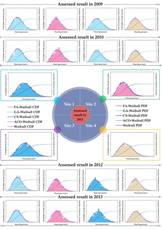
2.2.1. Assessment Results in a Single Year

The wind energy assessment is an important indicator to determine the potential of wind resources and describe the amount of wind energy at various wind speed values in a particular location. In a study of the wind energy assessment, the common parameter estimation methods include the method of moments estimate, maximum likelihood estimate, and least squares estimate, which have some disadvantages and limitations. For example, the method of moments estimate is simple where only knowing the moment of the population is sufficient and does not require knowledge of the population distribution. However, it can only be used in the distribution when the population origin moment exists, and the moment only has some of the information. This method only has good performance when the sample size is large. The maximum likelihood estimation (MLE) is a method of estimating the parameters of a statistical model according to observations by finding the parameter values that maximize the likelihood of making the observations given the parameters. However, the maximum likelihood estimation must incorporate the sample distribution. It is more complicated to incorporate the likelihood equations, which often obtains the approximate solution by computer iterative computation. The maximum likelihood estimation is complex and may lead to multi-optimal solutions or non-optimal solutions. The least squares can be applied to estimate linear and nonlinear relationships. When applying the least square to estimate the parameters of models, the observed data do not require information about the probability and statistics method. However, the least square has two kinds of defects. If the noise of model is colored noise, the estimation result of the least square is a biased estimation; with increasing data size, “data saturation” will appear. The Bayesian parameter estimation must know the distribution of the random error. When the sample size is small, prior probability has a significant influence on the estimation result (the result of maximum likelihood estimation, method of moments estimate, least square estimate and Bayesian parameter estimation in AppendixA). In summary, in this paper, the effectiveness of four optimization algorithms (Firefly Algorithm, Genetic Algorithm, Ant Colony Algorithm and Cuckoo Search Algorithm) is evaluated to determine the shape (k) and scale (c) parameters of the Weibull distribution function for calculating the wind power density. By comparing the assessment results, the swarm intelligent algorithm showed an effective assessment performance.









Figure 1.PDF fitting results in the single year from 2009 to 2013

With the PDF fitting results, in this paper, the following four error evaluation criteria (showed in Equations (5)–(7)) are adopted to evaluate the assessment performance:

MAE = 1

n n

∑

SSE = n

∑

(yi−yˆi)2 (6)

RMSE =

s 1 n

n

∑

(yi−yˆi)2 (7)

R2 = n

∑

i=1

(yi−y)2− n

∑

i=1

(yi−yˆi)2 n

∑

i=1

(yi−y)2

(8)

whereyiis the observed value, ˆyimeans the forecasted value, andyis calculated byy = n

∑

i=1 yi/n.

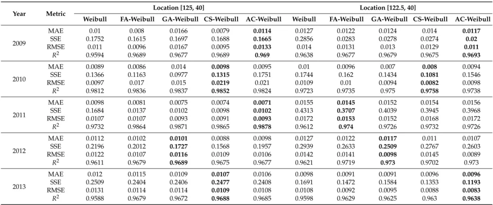
Table2provides the assessment performance evaluation results in a single year from 2009 to 2013 of the four optimization algorithms on a yearly basis in terms of MAE, RMSE, SSE andR2, respectively. As seen from Table2, although the presented descriptive statistics provide meaningful statistical analysis, especially regarding the distribution of the wind speed, they cannot be solely used to judge the precision level of each optimization algorithm for estimating the parameters of Weibull distribution. Therefore, the different evaluation criteria introduced by Equations (5)–(8) are employed to appraise the performances of the four selected parameter estimation optimization algorithms. It is meaningful that different statistical criterion supplies different useful views for comparing the optimization algorithms. As a result, the combination of all statistical indicators provides an effective way to compare the different parameter estimation optimization algorithms for wind power assessment. The effectivity of the assessed wind power density values changes when the parameter estimation optimization algorithms change. This is apparent for each research site when the four optimization algorithms of CS, GA, FA and AC are utilized to estimate the parameters of Weibull distribution. This conclusion is drawn from the low error values and highR2and SSE values. On the other hand, the lowest agreement levels are attained when the four algorithms are applied forkandcparameter calculations. According to the statistical results in Table2, for the four sites Chinese wind farm sites, the best results for calculating the wind speed density are achieved when the four optimization algorithms are employed to compute thekandcparameters. For each gate station site, the most precise results are obtained using the different optimization algorithms [20].

2.2.2. Seasonal and Whole Five-Year Assessment Results

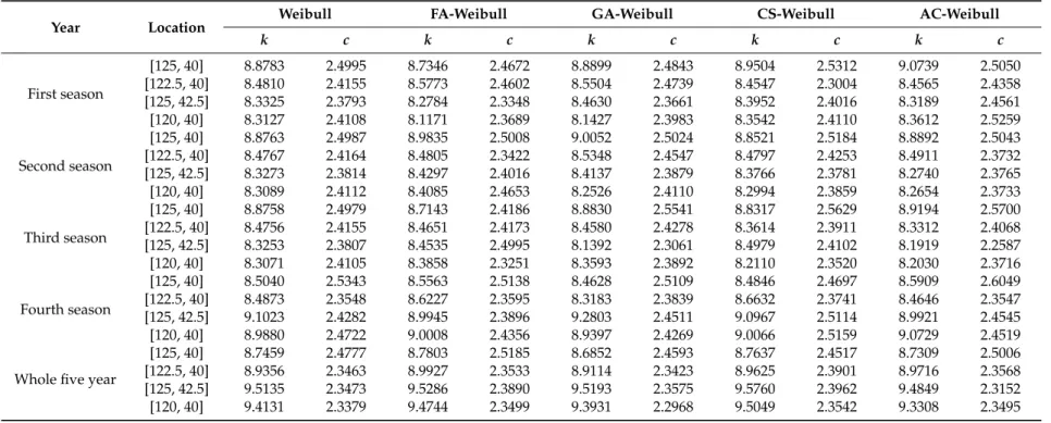
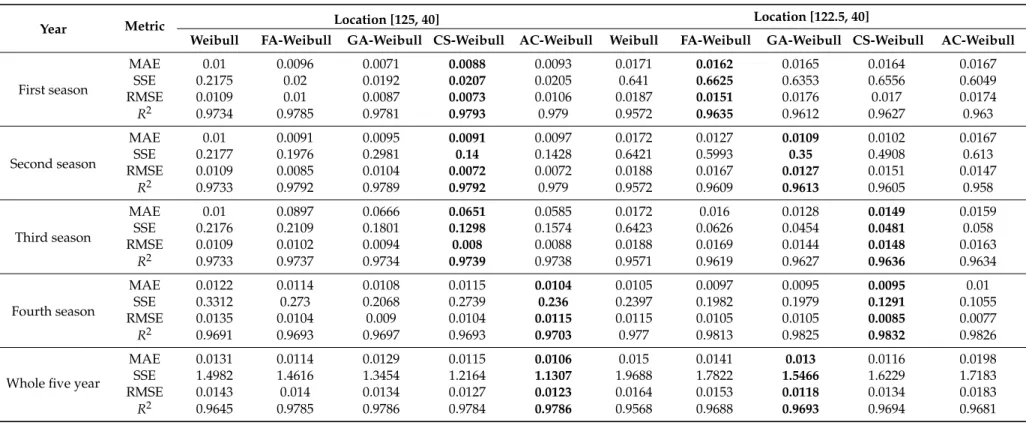
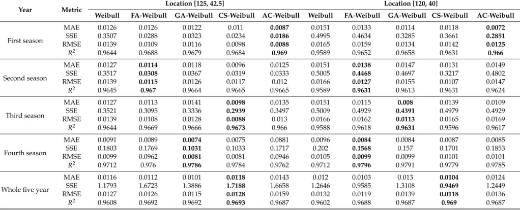
Considering that wind speed data may be vastly different in different years, this section provides seasonal and whole five-year wind energy assessment results by comprehensively using the wind speed data in the five years from 2009 to 2013. Similarly, Table3lists the seasonal and whole five-year parameter estimation results, and Figure2and Table4present the PDF fitting and corresponding error results.

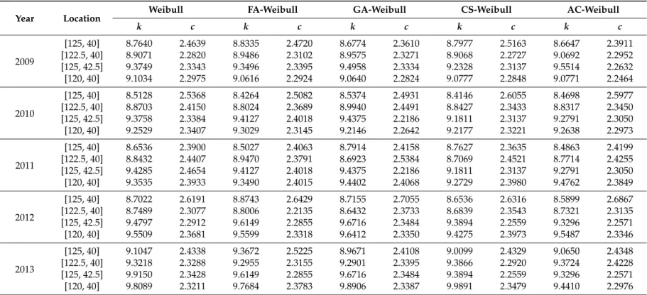
Table 1.Parameter estimation results in a single year from 2009 to 2013.

Year Location Weibull FA-Weibull GA-Weibull CS-Weibull AC-Weibull

k c k c k c k c k c

2009

[125, 40] 8.7640 2.4639 8.8335 2.4720 8.6774 2.3610 8.7977 2.5163 8.6647 2.3911 [122.5, 40] 8.9071 2.2820 8.9486 2.3102 8.9575 2.3271 8.9068 2.2727 9.0692 2.2952 [125, 42.5] 9.3749 2.3343 9.3496 2.3395 9.4958 2.3334 9.2328 2.3137 9.5514 2.2632 [120, 40] 9.1034 2.2975 9.0616 2.2924 9.0640 2.2824 9.0777 2.2848 9.0771 2.2464

2010

[125, 40] 8.5128 2.5368 8.4264 2.5082 8.5374 2.4931 8.4146 2.6055 8.4698 2.5977 [122.5, 40] 8.8703 2.4150 8.8024 2.3689 8.9940 2.4491 8.8427 2.3433 8.8317 2.3450 [125, 42.5] 9.3758 2.3384 9.4127 2.4018 9.4375 2.2186 9.1811 2.3137 9.2791 2.3050 [120, 40] 9.2529 2.3407 9.3029 2.3145 9.2146 2.2642 9.2177 2.3221 9.2638 2.2973

2011

[125, 40] 8.6536 2.3900 8.5027 2.4063 8.7914 2.4158 8.7627 2.3635 8.4863 2.4199 [122.5, 40] 8.8432 2.4407 8.9470 2.3791 8.6923 2.5384 8.7069 2.4521 8.7714 2.4255 [125, 42.5] 9.4285 2.4654 9.4127 2.4018 9.4375 2.2186 9.1811 2.3137 9.2791 2.3050 [120, 40] 9.3535 2.3933 9.3490 2.4015 9.4402 2.4068 9.2729 2.3980 9.4762 2.3849

2012

[125, 40] 8.7022 2.6191 8.8743 2.6429 8.7155 2.7055 8.6536 2.6316 8.5899 2.6867 [122.5, 40] 8.7489 2.3077 8.8006 2.2135 8.6432 2.3733 8.6839 2.3543 8.7321 2.3135 [125, 42.5] 9.4797 2.2912 9.6149 2.2855 9.6716 2.3484 9.3894 2.2559 9.3296 2.2571 [120, 40] 9.5509 2.3681 9.5599 2.3318 9.6412 2.3350 9.4275 2.3973 9.5487 2.3346

2013

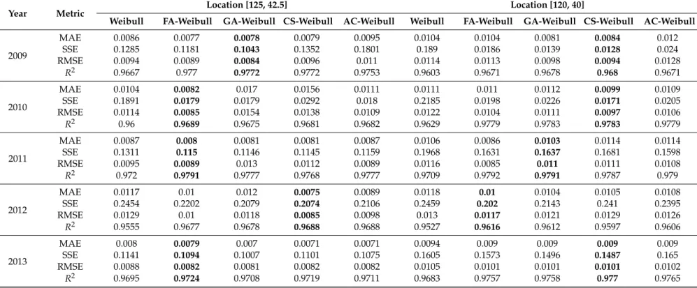
Table 2.Assessment error results in a single year from 2009 to 2013.

Year Metric Location [125, 40] Location [122.5, 40]

Weibull FA-Weibull GA-Weibull CS-Weibull AC-Weibull Weibull FA-Weibull GA-Weibull CS-Weibull AC-Weibull

2009

MAE 0.01 0.008 0.0166 0.0079 0.0114 0.0127 0.0122 0.0124 0.014 0.0117

SSE 0.1752 0.1615 0.1697 0.1688 0.1665 0.2856 0.0283 0.0278 0.0274 0.02

RMSE 0.011 0.0096 0.0167 0.0095 0.0133 0.014 0.0131 0.013 0.0129 0.011

R2 0.9594 0.9689 0.9677 0.9689 0.969 0.9638 0.9677 0.9679 0.9675 0.9693

2010

MAE 0.0089 0.0086 0.014 0.0098 0.0095 0.01 0.0096 0.007 0.008 0.0094

SSE 0.1366 0.1163 0.0977 0.1315 0.1751 0.1744 0.162 0.1434 0.1081 0.1546

RMSE 0.0097 0.017 0.015 0.0219 0.021 0.0109 0.01 0.0094 0.0082 0.0098

R2 0.9812 0.9836 0.9837 0.9852 0.9824 0.9723 0.9735 0.975 0.9758 0.9738

2011

MAE 0.0098 0.0081 0.0075 0.0074 0.0071 0.0155 0.0145 0.0152 0.0154 0.0156

SSE 0.1684 0.0137 0.0102 0.0098 0.0102 0.4313 0.3707 0.4039 0.3945 0.3968

RMSE 0.0107 0.0107 0.0093 0.0091 0.0093 0.0172 0.0153 0.0152 0.0168 0.0172

R2 0.9732 0.9864 0.9871 0.9865 0.9878 0.9612 0.974 0.9726 0.9732 0.9726

2012

MAE 0.0112 0.0102 0.0101 0.0088 0.0098 0.0127 0.0122 0.0117 0.011 0.0107

SSE 0.2196 0.2012 0.1727 0.1568 0.1957 0.2939 0.2633 0.2509 0.2767 0.2603

RMSE 0.0122 0.0107 0.0116 0.0109 0.0106 0.0142 0.0141 0.0098 0.0145 0.0089

R2 _{0.9611 0.9679 0.9689 0.9675 0.9677 0.9621 0.9719 0.973 0.9702 0.973}

2013

MAE 0.012 0.0115 0.0109 0.0107 0.0106 0.0098 0.0091 0.0091 0.0096 0.0096

SSE 0.2509 0.2404 0.2406 0.2477 0.2408 0.1691 0.1472 0.1584 0.1353 0.1193

RMSE 0.0131 0.0114 0.0114 0.0109 0.0108 0.0108 0.0092 0.0095 0.0088 0.0083

Table 2.Cont.

Year Metric Location [125, 42.5] Location [120, 40]

Weibull FA-Weibull GA-Weibull CS-Weibull AC-Weibull Weibull FA-Weibull GA-Weibull CS-Weibull AC-Weibull

2009

MAE 0.0086 0.0077 0.0078 0.0079 0.0095 0.0104 0.0104 0.0081 0.0084 0.012

SSE 0.1285 0.1181 0.1043 0.1352 0.1801 0.189 0.0186 0.0139 0.0128 0.024

RMSE 0.0094 0.0089 0.0084 0.0096 0.011 0.0114 0.0113 0.0098 0.0094 0.0128

R2 0.9667 0.977 0.9772 0.9772 0.9753 0.9603 0.9671 0.9678 0.968 0.9671

2010

MAE 0.0104 0.0082 0.017 0.0156 0.0111 0.0111 0.011 0.0112 0.0099 0.0109

SSE 0.1891 0.0179 0.0179 0.0292 0.018 0.2185 0.0198 0.0226 0.0171 0.0205

RMSE 0.0114 0.0085 0.0154 0.0138 0.0109 0.0122 0.0104 0.0111 0.0097 0.0106

R2 _{0.96 0.9689 0.9675 0.9681 0.9682 0.9629 0.9779 0.9783 0.9783 0.9779}

2011

MAE 0.0087 0.008 0.0081 0.0081 0.0087 0.0106 0.0086 0.0103 0.0114 0.0114

SSE 0.1311 0.115 0.1146 0.1145 0.1159 0.1968 0.1631 0.1637 0.1681 0.1598

RMSE 0.0095 0.0089 0.013 0.0112 0.0089 0.0116 0.0085 0.011 0.0111 0.0108

R2 _{0.972 0.9791 0.9777 0.9768 0.9777 0.9709 0.9792 0.9791 0.9787 0.979}

2012

MAE 0.0117 0.01 0.012 0.0075 0.0089 0.0118 0.01 0.0104 0.0105 0.0108

SSE 0.2454 0.2202 0.2079 0.2074 0.2106 0.2459 0.202 0.2143 0.241 0.2395

RMSE 0.0129 0.01 0.0118 0.0085 0.0098 0.013 0.0117 0.0121 0.0129 0.0126

R2 0.9555 0.9677 0.9678 0.9688 0.9688 0.9527 0.9616 0.9612 0.9597 0.9606

2013

MAE 0.008 0.0079 0.007 0.0071 0.0071 0.0094 0.009 0.009 0.009 0.009

SSE 0.1141 0.1094 0.1007 0.1101 0.1075 0.1605 0.1573 0.1496 0.1487 0.165

RMSE 0.0088 0.0082 0.0081 0.0082 0.0082 0.0105 0.0101 0.0101 0.0101 0.0102

Table 3.Seasonal and whole five-year parameter estimation results.

Year Location Weibull FA-Weibull GA-Weibull CS-Weibull AC-Weibull

k c k c k c k c k c

First season

[125, 40] 8.8783 2.4995 8.7346 2.4672 8.8899 2.4843 8.9504 2.5312 9.0739 2.5050 [122.5, 40] 8.4810 2.4155 8.5773 2.4602 8.5504 2.4739 8.4547 2.3004 8.4565 2.4358 [125, 42.5] 8.3325 2.3793 8.2784 2.3348 8.4630 2.3661 8.3952 2.4016 8.3189 2.4561 [120, 40] 8.3127 2.4108 8.1171 2.3689 8.1427 2.3983 8.3542 2.4110 8.3612 2.5259

Second season

[125, 40] 8.8763 2.4987 8.9835 2.5008 9.0052 2.5024 8.8521 2.5184 8.8892 2.5043 [122.5, 40] 8.4767 2.4164 8.4805 2.3422 8.5348 2.4547 8.4797 2.4253 8.4911 2.3732 [125, 42.5] 8.3273 2.3814 8.4297 2.4016 8.4137 2.3879 8.3766 2.3781 8.2740 2.3765 [120, 40] 8.3089 2.4112 8.4085 2.4653 8.2526 2.4110 8.2994 2.3859 8.2654 2.3733

Third season

[125, 40] 8.8758 2.4979 8.7143 2.4186 8.8830 2.5541 8.8317 2.5629 8.9194 2.5700 [122.5, 40] 8.4756 2.4155 8.4651 2.4173 8.4580 2.4278 8.3614 2.3911 8.3312 2.4068 [125, 42.5] 8.3253 2.3807 8.4535 2.4995 8.1392 2.3061 8.4979 2.4102 8.1919 2.2587 [120, 40] 8.3071 2.4105 8.3858 2.3251 8.3593 2.3892 8.2110 2.3520 8.2030 2.3716

Fourth season

[125, 40] 8.5040 2.5343 8.5563 2.5138 8.4628 2.5109 8.4846 2.4697 8.5909 2.6049 [122.5, 40] 8.4873 2.3548 8.6227 2.3595 8.3183 2.3839 8.6632 2.3741 8.4646 2.3547 [125, 42.5] 9.1023 2.4282 8.9945 2.3896 9.2803 2.4511 9.0967 2.5114 8.9921 2.4545 [120, 40] 8.9880 2.4722 9.0008 2.4356 8.9397 2.4269 9.0066 2.5159 9.0729 2.4519

Whole five year

Table 4.Seasonal and whole five-year assessment error results.

Year Metric Location [125, 40] Location [122.5, 40]

Weibull FA-Weibull GA-Weibull CS-Weibull AC-Weibull Weibull FA-Weibull GA-Weibull CS-Weibull AC-Weibull

First season

MAE 0.01 0.0096 0.0071 0.0088 0.0093 0.0171 0.0162 0.0165 0.0164 0.0167

SSE 0.2175 0.02 0.0192 0.0207 0.0205 0.641 0.6625 0.6353 0.6556 0.6049

RMSE 0.0109 0.01 0.0087 0.0073 0.0106 0.0187 0.0151 0.0176 0.017 0.0174

R2 0.9734 0.9785 0.9781 0.9793 0.979 0.9572 0.9635 0.9612 0.9627 0.963

Second season

MAE 0.01 0.0091 0.0095 0.0091 0.0097 0.0172 0.0127 0.0109 0.0102 0.0167

SSE 0.2177 0.1976 0.2981 0.14 0.1428 0.6421 0.5993 0.35 0.4908 0.613

RMSE 0.0109 0.0085 0.0104 0.0072 0.0072 0.0188 0.0167 0.0127 0.0151 0.0147

R2 _{0.9733 0.9792 0.9789 0.9792 0.979 0.9572 0.9609 0.9613 0.9605 0.958}

Third season

MAE 0.01 0.0897 0.0666 0.0651 0.0585 0.0172 0.016 0.0128 0.0149 0.0159

SSE 0.2176 0.2109 0.1801 0.1298 0.1574 0.6423 0.0626 0.0454 0.0481 0.058

RMSE 0.0109 0.0102 0.0094 0.008 0.0088 0.0188 0.0169 0.0144 0.0148 0.0163

R2 _{0.9733 0.9737 0.9734 0.9739 0.9738 0.9571 0.9619 0.9627 0.9636 0.9634}

Fourth season

MAE 0.0122 0.0114 0.0108 0.0115 0.0104 0.0105 0.0097 0.0095 0.0095 0.01

SSE 0.3312 0.273 0.2068 0.2739 0.236 0.2397 0.1982 0.1979 0.1291 0.1055

RMSE 0.0135 0.0104 0.009 0.0104 0.0115 0.0115 0.0105 0.0105 0.0085 0.0077

R2 0.9691 0.9693 0.9697 0.9693 0.9703 0.977 0.9813 0.9825 0.9832 0.9826

Whole five year

MAE 0.0131 0.0114 0.0129 0.0115 0.0106 0.015 0.0141 0.013 0.0116 0.0198

SSE 1.4982 1.4616 1.3454 1.2164 1.1307 1.9688 1.7822 1.5466 1.6229 1.7183

RMSE 0.0143 0.014 0.0134 0.0127 0.0123 0.0164 0.0153 0.0118 0.0134 0.0183

Table 4.Cont.

Year Metric Location [125, 42.5] Location [120, 40]

Weibull FA-Weibull GA-Weibull CS-Weibull AC-Weibull Weibull FA-Weibull GA-Weibull CS-Weibull AC-Weibull

First season

MAE 0.0126 0.0126 0.0122 0.011 0.0087 0.0151 0.0133 0.0114 0.0118 0.0072

SSE 0.3507 0.0288 0.0323 0.0234 0.0186 0.4995 0.4634 0.3285 0.3661 0.2851

RMSE 0.0139 0.0109 0.0116 0.0098 0.0088 0.0165 0.0159 0.0134 0.0142 0.0125

R2 0.9644 0.9688 0.9679 0.9684 0.969 0.9589 0.9652 0.9658 0.9631 0.966

Second season

MAE 0.0127 0.0114 0.0118 0.0096 0.0125 0.0151 0.0138 0.0147 0.0131 0.0149

SSE 0.3517 0.0308 0.0367 0.0319 0.0333 0.5005 0.4468 0.4697 0.3217 0.4802

RMSE 0.0139 0.0115 0.0126 0.0117 0.012 0.0166 0.0127 0.0155 0.0107 0.0147

R2 _{0.9645 0.967 0.9664 0.9665 0.9665 0.9589 0.9631 0.9613 0.9631 0.9624}

Third season

MAE 0.0127 0.0113 0.0141 0.0098 0.0135 0.0151 0.0115 0.008 0.0139 0.0109

SSE 0.3521 0.3095 0.3336 0.2939 0.3497 0.5009 0.4929 0.4391 0.4979 0.4929

RMSE 0.0139 0.0108 0.0128 0.0088 0.013 0.0166 0.0162 0.0113 0.0165 0.0169

R2 _{0.9644 0.9669 0.9666 0.9673 0.966 0.9588 0.9618 0.9631 0.9596 0.9617}

Fourth season

MAE 0.0091 0.0089 0.0074 0.0075 0.0881 0.0096 0.0084 0.0084 0.0087 0.0085

SSE 0.1803 0.1769 0.1031 0.1033 0.1717 0.202 0.1568 0.157 0.1701 0.1853

RMSE 0.0099 0.0962 0.0081 0.0081 0.0946 0.0105 0.0099 0.0099 0.0101 0.0101

R2 0.9712 0.976 0.9786 0.9784 0.9762 0.9712 0.9796 0.9791 0.9779 0.9785

Whole five year

MAE 0.0116 0.0112 0.0101 0.0118 0.0143 0.012 0.0103 0.013 0.0104 0.0124

SSE 1.1793 1.6723 1.3886 1.7188 1.6658 1.2646 0.9585 1.3108 0.9469 1.2449

RMSE 0.0127 0.0126 0.0115 0.0128 0.0159 0.0132 0.0119 0.0139 0.0118 0.0136

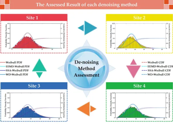
Figure 2. Seasonal PDF and whole five-year fitting results.

Figure 2.Seasonal PDF and whole five-year fitting results.

parameter estimation algorithm for optimizing the wind power density in each year and season. For Site 3, the AC showed poor performance for the annual wind power density distribution, and the FA was recognized as a more appropriate method. For Site 4, both the FA and GA perform better for the seasonal wind power density. The suggested parameter estimation methods have excellent performance for representing the distribution of seasonal and annual wind power density as well as determining different statistical properties of the power density [20].

3. Connection between Energy Assessment and Forecasting

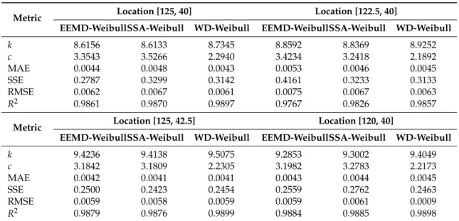
In recent years, the de-noising method is widely used to preprocess wind speed time series, such as the Ensemble Empirical Mode Decomposition (EEMD), Singular Spectrum Analysis (SSA), and the Wavelet decomposition (WD). Thus far, there is no effective way to choose which de-noising methods should be used to address the original wind speed time series. In this section, the wind energy assessment method with the smallest error values is used to choose the best de-nosing method to pre-process the wind speed time series.

Figure3presents the PDF fitting results obtained by three different de-noising methods for the four sites, and Table5shows the parameter estimation and error results of the different de-nosing wind speed time series. As seen from Figure3and Table5, theR2_{values from Site 1 to Site 4 in the WD} de-noising method are all closest to 1. Assessment results obtained by the three de-noising models show that the MAE values of the WD de-noising method is the smallest. In this paper, the WD de-noising method is adopted to preprocess the original wind speed to improve the forecasting accuracy.

Figure 3. PDF fitting results obtained by three different de-noising methods for the four sites.

Table 5.Assessment results of each de-noising wind speed time series.

Metric Location [125, 40] Location [122.5, 40]

EEMD-WeibullSSA-Weibull WD-Weibull EEMD-WeibullSSA-Weibull WD-Weibull

k 8.6156 8.6133 8.7345 8.8592 8.8369 8.9252

c 3.3543 3.5266 2.2940 3.4234 3.2418 2.1892

MAE 0.0044 0.0048 0.0043 0.0053 0.0046 0.0045

SSE 0.2787 0.3299 0.3142 0.4161 0.3233 0.3133

RMSE 0.0062 0.0067 0.0061 0.0075 0.0067 0.0063

R2 0.9861 0.9870 0.9897 0.9767 0.9826 0.9857

Metric Location [125, 42.5] Location [120, 40]

EEMD-WeibullSSA-Weibull WD-Weibull EEMD-WeibullSSA-Weibull WD-Weibull

k 9.4236 9.4138 9.5075 9.2853 9.3002 9.4049

c 3.1842 3.1809 2.2305 3.1982 3.2783 2.2173

MAE 0.0042 0.0041 0.0041 0.0043 0.0044 0.0045

SSE 0.2500 0.2423 0.2454 0.2559 0.2762 0.2463

RMSE 0.0059 0.0058 0.0059 0.0059 0.0061 0.0009

R2 0.9879 0.9876 0.9899 0.9884 0.9885 0.9898

4. Proposed Integrated Forecasting Framework and Forecasting Results

In this section, three basic neural network forecasting models are first introduced; then, the integrated forecasting framework proposed in this paper is shown. Finally, the forecasting results obtained by the new proposed forecasting framework are analyzed.

4.1. Basic Neural Network Forecasting Models

Artificial neural networks are usually used to forecast fields as they can approximate nonlinear functions with arbitrary accuracy. Three neural network models are introduced in this paper for the wind speed forecasting application.

4.1.1. Back Propagation Neural Network

The back propagation neural network (BPNN) [21] is a multilayer feed-forward neural network. The two main features that should be considered in BPNN are the feed-forward signal and back propagated error. In the feed-forward process, the signal is passed layer-by-layer from the input layer to the hidden layer and then to the output layer. The state of the neurons only impacts the neurons in the adjacent next layer. If the output in the output layer is not expected, back propagation starts.

SupposeX1,X2, . . . ,Xnare the input values of the BPNN;Y1,Y2, . . . ,Ymare the corresponding

output values; andωij andωjk are the weights, the BPNN can be viewed as a non-linear function

and the input values and output values can be regarded as the independent and dependent variables. The BPNN structure in Figure4is the expression of the function mapping relation fromnindependent variables tomdependent variables.

The network training is the main task of the BPNN. Through the training operation, the BPNN has capacity for associative memory and forecasting. The training process of the BPNN includes the following steps:

Step 1:Network initialization. Based on the practical problem, determine the number of nodes in the input, hidden and output layers. Then, initialize the following values: the connection weightsωij

Step 2: The output calculation of the hidden layer. According to the input vector X= (X1,X2, . . . ,Xn), the connection weights ωij between the input and hidden layers and the

threshold valueθjin the hidden layer as well as the output of the hidden layer can be calculated by

Equation(9):

Hj = f l

∑

ωijxi−θj !

(9)

wherelis the number of nodes in the hidden layer and f(·)is the transfer function of the hidden layer, which has a variety of expression forms. In this research, the following form is adopted in Equation (10):

f(x) = 1

1+e−x (10)

Step 3:The output calculation of the output layer. According to the outputHjof the hidden layer,

the connection weightsωjkbetween the hidden layer and output layer, and the threshold valueθjin

the output layer, the forecasting output of the BPNN can be expressed as Equation (11):

Yk = g

∑

ωjkHj−θk !

(11)

whereg(·)is the transfer function from the hidden layer to the output layer, which is defined as Equation (12) in this research:

g(x) = 1

1+e−x (12)

Step 4:Error calculation. With the predicted outputY= (Y1,Y2, . . . ,Ym)and the desired output DY= (DY1,DY2, . . . ,DYm), the forecasting error of the network is computed by Equation (13):

e= 1

2P P

∑

m

∑

DY_jp−Y_jp2 (13)

wherePis the number of the input and output pairs.

Step 5:Weights update. Update the connection weightsωijandωjkby Equations (14) and (15):

ωjk =ωjk+ηδkHj (14)

ωij =ωij+ηδjXi (15)

whereηis the learning rate, and shows Equations (16) and (17)

δk =Yk(1−Yk) (DYk−Yk) (16)

δj=Hj 1−Hj

∑

ωjkδk (17)

Step 6:Threshold update. By using the forecasting error of the network, the threshold is updated by Equations (18) and (19):

θk =θk−ηδk (18)

θj=θj−ηδj (19)

Figure 4. Three optimized neural networks.

 











_





























 















Figure 4.Three optimized neural networks.

4.1.2. Wavelet Neural Network

The Wavelet Neural Network (WNN) [22] is a neural network type that is constructed on the basis of the BPNN topology, and the wavelet basis function is regarded as the transfer function of the hidden layer nodes. In this type of network, the signal is transferred feed-forward, while the error is transferred back-forward. SupposeX1,X2, . . . ,Xnare the inputs of the network,Y1,Y2, . . . ,Ymare the

forecasted output, andωijandωjk are the weights, the output of the hidden layer can be represented

by Equation (20)

hj=h 

  

n

∑

i=1

ωijXi−bj aj



  

(20)

wherehjis the output of thejth hidden layer node,ωijis the connection weight between the input and

hidden layers,h(·)is the wavelet function,bjis the shift factor of the wavelet function, andajis the

stretch factor wavelet function.

The forecasted value of the output layer can be calculated by Equation (21):

yk= l

∑

ωjkhj, k=1, 2, . . . ,m (21)

whereωjk is the weight between the hidden and output layers, hj is the output of thejth hidden

The process of the WNN algorithm is as follows:

Step 1:Network initialization. Randomly initialize the stretch factorak, shift factorbk, network

connection weightsωijandωjk, and network learning rateη.

Step 2:Sample classification. Divide the samples into the training and testing samples, which are used to train the network and test the forecasting accuracy of the network, respectively.

Step 3:Output prediction. Input the training sample into the network and calculate the predicted output of the network as well as the error between the network output and desired output.

Step 4: Weight correction. Correct the network weights and parameters in the wavelet function according to the calculated error values, helping the network predicted values approach the expected values.

Step 5: Algorithm termination judgment. Determine whether the algorithm termination is satisfied; if not, return to Step 3.

4.1.3. Elman Neural Network

ENN [23] is generally divided into four layers, input, hidden, context and output layers. The connections between the input, hidden and output layers are similar to the feed-forward network. The nodes in the input layer only play a signal transmission role, while those in the output layer have a linear weighted effect. The transfer function of the hidden layer can be either linear or nonlinear, and the context layer, which is also known as the undertake or state layer, is used to remember the previous output of the hidden layer and return it to the network input so it can be considered a single-step delay operator.

Through the delay and storage of the context layer, the output of the hidden layer can be self-connected to the input of the hidden layer. This self-connection approach makes the network sensitive to the historical data and increases the capacity of the network to address the dynamic information, which can then achieve the dynamic modeling purpose. In addition, the ENN can approximate any nonlinear map with arbitrary precision without considering the specific form of the external noise impact on the system. Therefore, given the input and output pair of the system, the system can be modeled.

4.2. Structure of the Proposed Integrated Forecasting Framework

Algorithm 3:Three Neural Networks Optimized by the CS Algorithm

Input:

x(s0) =

x(0)(1),x(0)(2), . . . ,x(0)(q)—a sequence of training data. x(p0) =

x(0)_{(q + 1),x}(0)_{(q + 2), . . . ,x}(0)_{(q + d)—a sequence of verifying data}

Output:

xb—the value ofxwith the best fitness value in population of nests

Fitness Function:x(k) = f(ω1xc(k) + ω2(u(k−1))) (ENN) f(net) = _1+e1−net (BPNN)

h(j) =hj 

 

k

∑

i=1ωij

x−bj

a_j 



 (WNN)

Parameters:

Num Cuckoos = 50 number of initial population

Min Number Of Eggs = 2; minimum number of eggs for each cuckoo Max Number Of Eggs = 4; maximum number of eggs for each cuckoo Max Iter = 200; maximum iterations of the Cuckoo Algorithm Knn Cluster Num = 1; number of clusters that we want to make Motion Coeff = 20; Lambda variable in COA paper, default = 2 accuracy = 0×10−10; How much accuracy in answer is needed

Max Num Of Cuckoos = 20; maximum number of cuckoos that can live at the same time Radius Coeff = 0.05; Control parameter of egg laying

Cuckoo Pop Variance = 1×10−10; population variance that cuts the optimization 1:/*Initialize population ofnhost nestsxi(i= 1, 2, ...,n) randomly*/

2:FOR EACHi: 1≤i≤nDO

3: Evaluate the corresponding fitness functionF_i 4:END FOR

5:WHILE(g<GenMax)DO

6: /* Get new nests byLévyflights */ 7:FOR EACHi: 1≤i≤nDO 8:xL=xi+α⊕Levy(λ);

9:END FOR

10:FOR EACHi: 1≤i≤nDO 11: ComputeFL

12:IF(FL<Fi)THEN

13:xi←xL;

14:END IF 15:END FOR 16: ComputeFL

17:/*Update best nestxpof thedgeneration*/

18:IF (Fp<Fb)THEN

19:xb←xp;

Algorithm 4:Three Neural Networks Optimized by the AC Optimization Algorithm

Input:

x(0)s =

x(0)(1),x(0)(2), . . . ,x(0)(q)—a sequence of training data.

x(0)p =

x(0)(q+1),x(0)(q+2), . . . ,x(0)(q+d)—a sequence of verifying data

Output:

xb—the value ofxwith the best fitness value in population of nests Fitness Function:x(k) = f(ω1xc(k) +ω2(u(k−1))) (ENN)

f(net) = 1

1+e−net (BPNN)

h(j) =hj 

 

k

∑

i=1

ωijx−bj

aj    (WNN) Parameters: Maximum iterations:50 The number of ant:30

Parameters of the important degree of information elements:1 Parameters of the important degree of the Heuristic factor:5 Parameters of the important degree of the heuristic factor:0.1 Pheromone increasing intensity coefficient:100

NC_max—Maximum iterations:50 m—The number of ant:30

Alpha—Parameters of the important degree of information elements:1 Beta—Parameters of the important degree of the Heuristic factor:5 Rho—Parameters of the important degree of the heuristic factor:0.1 Q—Pheromone increasing intensity coefficient:100

1: /*Initializepopsizecandidates with the values between 0 and 1*/ 2:FOR EACHi1≤i≤nDO

3:α1_i =rand(m,n)

4:END FOR

5:P=

αiter_i : 1≤i≤popsize

6:iter= 1; Evaluate the corresponding fitness functionFi

7: /* Find the best value of repeatedly until the maximum iterations are reached. */ 8:WHILE.(iter≤itermax)DO

9: /* Find the best fitness value for each candidates */ 10:FOR EACHαiter_i ∈PDO

11: Buildneuralnetworkby usingx(0)s with theαiteri value 12: Calculate ˆx(0)p =

ˆ

x(0)_p+1, ˆx(0)_p+2, . . . , ˆx(0)_p+3byneuralnetwork 13: /*Choose the best fitness value of theithcandidate in history */ 14:IF(pBesti>fitness(αiteri ))THEN

15:pBesti=fitness(αiteri ) 16:END IF

17:END FOR

18: /* Choose the candidate with the best fitness value of all the candidates */ 19:FOR EACHαiter_i ∈PDO

20:IF(gBest>pBesti)THEN

21:gBest = pBesti= xkt+1=xgbest±:t=1, 2,· · ·,T 22:αbest=αiteri

23:END IF

Algorithm 4:Cont.

25: /*Update the values of all the candidates by using ACO’s evolution equations.*/ 26:FOR EACHαiter_i ∈PDO

27:αt+1 = 0.1 × αt

28:xgbest = xgbest + (xgbest × 0.01)→ (

i f f(xgbest) − f(xgbest) ≤ →the sign is(+)

i f f(xgbest) − f(xgbest) ≤ →the sign is(−)

29:END FOR

30:P =

αiter_i : 1 ≤ i ≤ popsize 31:iter=iter+ 1

32:END WHILE

 

    







    









  

Figure 5. The flowchart of this proposed integrated forecasting model.

Figure 5.The flowchart of this proposed integrated forecasting model.

4.3. Wind Speed Forecasting Case Study

the inputs are also the de-noised wind speed data, and the output is the original testing output. However, the testing output is assumed to be unknown.

Figure6presents the data division results; in this paper, the training dataset window with length N =1008 is fixed according to the original time series. For example, suppose a study of the wind speed time series will be forecasted. Apart from the data division, the forecasting horizon is also an important index. In this paper, multi-step ahead forecasting with valuesh =1, 2, and 3 are analyzed, wherehis a prediction step.

Figure 6. Data division.

















1010 ... M+6 M+7 M+8 ... N+6 N+7 ... 1153 1009 ... M+5 M+6 M+7 ... N+5 N+6 ... 1152

1011 ... M+7 M+8 M+9 ... N+7 N+8 ... 1154

Testing dataset input Testing dataset output

...

2 ... M+1 M+2 M+3 ... N+1 N+2 ... 1004 1 ... M M+1 M+2 ... N N+1 ... 1003

5 ... M+4 M+5 M+6 ... N+4 N+5 ... 1008

Training dataset input Training dataset output

First layer Second layer Fifth layer One step prediction Two step prediction Three step prediction

...

Figure 6.Data division.

Related parameter initialization values in different neural networks are shown in Table6. Based on the error evaluation criteria, MAE, defined in Equation (5) and the following two forecasting error evaluation criteria shows in Equations (22) and (23), forecasting error values obtained by different neural networks are listed in Table7.

MSE= 1

n n

∑

(yi−yˆi)2 (22)

MAPE= 1

n n

∑

yi−yˆi yi

(23)

where yi and ˆyi are the actual and forecasted wind speed values, and n is the number of the

data samples.

Table 6.Related parameter initialization values in the neural networks.

WD-CS/AC-ENN Model WD-CS/AC-BPNN Model WD-CS/AC-WNN Model

WD-CS-ENN WD-AC-ENN WD-CS-BPNN WD-AC-BPNN WD-CS-WNN WD-AC-WNN

Number of input neuronsNi: 3

Number of input neuronsNi: 4

Number of input neuronsNi: 5

Number of input neuronsNi: 5

Number of input neuronsNi: 5

Number of input neuronsNi: 3

Number of hidden layer neuronsNj: 16

Number of hidden layer neuronsNj: 22

Number of hidden layer neuronsNj: 15

Number of hidden layer neuronsNj: 16

Number of hidden layer neuronsNj: 19

Number of hidden layer neuronsNj: 20

Number of output neuronsNk: 1

Number of output neuronsNk: 1

Number of output neuronsNk: 1

Number of output neuronsNk: 1

Number of output neuronsNk: 1

Number of output neuronsNk: 1

Maximum of iterative steps:1000

Maximum of iterative steps: 1000

Maximum of iterative steps: 1000

Maximum of iterative steps: 1000

Maximum of iterative steps: 1000

Maximum of iterative steps: 1000

Value of the learning rate: 0.01

Value of the learning rate: 0.01

Value of the learning rate: 0.01

Value of the learning rate: 0.01

Value of the learning rate: 0.01

Value of the learning rate: 0.01

Table 7.Forecasting error values of each model.

Horizon Criterion Single Model Model Optimized by the WD Model Optimized by the WD and CS Model Optimized by the WD and AC ENN BPNN WNN WD-ENN WD-BPNN WD-WNN WD-CS-ENN WD-CS-BPNN WD-CS-WNN WD-AC-ENN WD-AC-BPNN WD-AC-WNN

One-step-ahead

MAE 0.6387 0.5164 0.5424 0.5579 0.4067 0.2769 0.2842 0.2681 0.2168 0.3612 0.2845 0.3131

MSE 0.6951 0.4561 0.5503 0.5554 0.2913 0.1484 0.1545 0.1376 0.0851 0.2203 0.1636 0.1755

MAPE 0.0961 0.0770 0.0788 0.0832 0.0619 0.0593 0.0402 0.0379 0.0383 0.0534 0.0361 0.0371

Two-steps-ahead

MAE 0.6941 0.5360 0.5431 0.6405 0.4084 0.3622 0.3037 0.2844 0.2370 0.3793 0.3408 0.3489

MSE 0.8167 0.4987 0.5335 0.7155 0.4541 0.4546 0.506 0.4585 0.4557 0.4895 0.4399 0.4469

MAPE 0.1038 0.0790 0.0792 0.0953 0.0698 0.0646 0.0744 0.0698 0.0634 0.0728 0.0682 0.0684

Three-steps-ahead

MAE 0.7199 0.5535 0.5814 0.6815 0.4620 0.5285 0.3556 0.3192 0.3153 0.3553 0.2624 0.2850

MSE 0.9084 0.7310 0.7546 0.8149 0.7046 0.6995 0.6527 0.6042 0.6059 0.2117 0.1310 0.1569

Figure 7. One-step-ahead forecasting results obtained by different models.

Figure 7.One-step-ahead forecasting results obtained by different models.

Figure 8. Two-step-ahead forecasting results obtained by different models.

Figure 9. Three-steps-ahead forecasting results obtained by different models.

5. Conclusions

Effective wind energy potential assessment and forecasting for a particular site plays an indispensable role in the design, evaluation and scheduling of wind farms. In this paper, based on the CS and AC algorithms, two new wind energy assessment models, as well as six wind speed forecasting models, are proposed. First, the CS and AC algorithms are introduced to estimate the two unknown parameters in the Weibull distribution as well as improve the assessment accuracy. The four assessment error evaluation criteria sets of results demonstrate that the two newly proposed assessment models are effective and meaningful. Then, the best data pre-processing approach is selected according to the wind energy potential evaluation results and is adopted to process the wind speed time series. Finally, the CS and AC algorithms are used to optimize three neural networks—namely the ENN, BPNN and WNN—and the three sets of forecasting error evaluation criteria results demonstrate that the six newly proposed assessment models perform better than the original ones. Therefore, forecasting researchers can greatly benefit from data pre-processing and swarm intelligent optimization techniques and these data allow for significant improvements in accuracy.

Acknowledgments: The work was supported by the National Natural Science Foundation of China (Grant No. 11161041).

Author Contributions:Zhilong Wang and Chen Wang conceived and designed the experiments; Chen Wang performed the experiments; Zhilong Wang and Chen Wang analyzed the data; Zhilong Wang and Jie Wu wrote the paper and Chen Wang checked the whole paper.

Appendix A

Table A1.The result of method of moments estimate, maximum likelihood estimate, least squares estimate, Bayesian prior estimate and Bayesian posterior estimate.

[125, 40] [122.5, 40]

Parameter MM MLE LSE Bayesian Prior Bayesian Posterior MM MLE LSE Bayesian Prior Bayesian Posterior

2009

k 8.7667 8.7684 8.7686 8.775 8.7602 8.9165 8.9194 8.917 8.928 8.916

c 2.482 2.482 2.4575 2.4523 2.5002 2.3113 2.3113 2.3021 2.2635 2.3293

MAE 0.0115 0.0092 0.0206 0.008 0.0145 0.0128 0.0157 0.0153 0.0177 0.0133

SSE 0.1992 0.1649 0.2123 0.1696 0.1976 0.3635 0.0363 0.0309 0.0322 0.0224

RMSE 0.0121 0.0122 0.0216 0.011 0.0164 0.018 0.0161 0.0139 0.014 0.0127

R2 _{0.9439 0.9441 0.9419 0.942 0.9447 0.9511 0.9514 0.9503 0.9466 0.9527}

2010

k 8.5254 8.5267 8.525 8.5162 8.5189 8.906 8.9078 8.9062 8.9055 8.8965

c 2.5432 2.5432 2.5484 2.5332 2.5607 2.4737 2.4737 2.4714 2.3815 2.4949

MAE 0.0101 0.0086 0.0145 0.0109 0.0111 0.0123 0.0097 0.0078 0.0094 0.0106

SSE 0.1472 0.134 0.1083 0.1505 0.1851 0.1979 0.166 0.1644 0.1116 0.1758

RMSE 0.0116 0.0209 0.0193 0.0229 0.021 0.0119 0.0109 0.0111 0.0092 0.011

R2 _{0.8905 0.8908 0.8907 0.8885 0.8902 0.9056 0.9058 0.9054 0.8923 0.9068}

2011

k 8.6657 8.6678 8.6657 8.6688 8.6579 8.8481 8.85 8.8499 8.8562 8.8493

c 2.4147 2.4147 2.4153 2.3754 2.437 2.4617 2.4617 2.4396 2.4272 2.4713

MAE 0.0156 0.0136 0.0122 0.0138 0.013 0.0114 0.0118 0.0114 0.0107 0.0111

SSE 0.2727 0.2412 0.2745 0.2872 0.3014 0.2065 0.1801 0.1646 0.1663 0.1287

RMSE 0.015 0.012 0.0134 0.0131 0.0137 0.0125 0.011 0.012 0.0092 0.0084

R2 0.9386 0.9389 0.9386 0.935 0.9393 0.9615 0.9617 0.9604 0.96 0.9621

2012

k 8.6999 8.7006 8.707 8.7159 8.6974 8.7481 8.7507 8.7494 8.7627 8.7487

c 2.6504 2.6504 2.5806 2.5914 2.6551 2.3396 2.3396 2.3128 2.2814 2.3555

MAE 0.0171 0.0153 0.013 0.0145 0.014 0.0128 0.0114 0.0116 0.0139 0.0129

SSE 0.3563 0.3237 0.279 0.3263 0.304 0.1998 0.2063 0.1957 0.205 0.1392

RMSE 0.0189 0.0178 0.0176 0.0146 0.0118 0.014 0.0127 0.0118 0.0108 0.0123

R2 _{0.9522 0.9522 0.9451 0.9467 0.9525 0.9464 0.9466 0.9427 0.9386 0.9486}

2013

k 9.1137 9.1155 9.1173 9.1303 9.1136 9.3264 9.3291 9.328 9.3426 9.3066

c 2.4728 2.4728 2.4282 2.4069 2.4829 2.3573 2.3573 2.3302 2.3099 2.3895

MAE 0.015 0.0196 0.0156 0.0172 0.019 0.0122 0.0163 0.0151 0.0112 0.0154

SSE 0.3543 0.342 0.4021 0.3286 0.3146 0.3301 0.221 0.2597 0.2208 0.1968

RMSE 0.0196 0.0123 0.016 0.0154 0.0196 0.0157 0.0156 0.014 0.0124 0.0141

R2 _{0.9603 0.9604 0.9549 0.9527 0.9614 0.9534 0.9535 0.9494 0.9469 0.9563}

Frist season

k 8.8812 8.8827 8.8828 8.8854 8.8741 8.7847 8.786 8.7892 8.7987 8.7844

c 2.5116 2.5116 2.4928 2.4921 2.5293 2.5463 2.5463 2.4959 2.4757 2.5485

MAE 0.0149 0.0117 0.0138 0.0132 0.0106 0.0127 0.0108 0.0121 0.0104 0.0109

SSE 0.3556 0.3537 0.2258 0.3241 0.2447 0.296 0.2494 0.2022 0.1519 0.1361

RMSE 0.0164 0.0105 0.0112 0.0126 0.0143 0.0118 0.0118 0.0132 0.0108 0.0095

Table A1.Cont.

[125, 40] [122.5, 40]

Parameter MM MLE LSE Bayesian Prior Bayesian Posterior MM MLE LSE Bayesian Prior Bayesian Posterior

Second season

k 8.4894 8.4913 8.4912 8.499 8.4896 9.1952 9.1979 9.1971 9.2135 9.1931

c 2.4451 2.4451 2.4199 2.3963 2.4474 2.3463 2.3463 2.3114 2.2909 2.3632

MAE 0.0138 0.0163 0.0159 0.0143 0.0142 0.0148 0.015 0.0108 0.0108 0.0152

SSE 0.4155 0.3622 0.2766 0.4315 0.2447 0.2865 0.2507 0.2978 0.1967 0.162

RMSE 0.0162 0.0141 0.0102 0.0134 0.0144 0.0151 0.0123 0.0142 0.0121 0.0102

R2 0.9688 0.9689 0.9674 0.966 0.969 0.9416 0.9417 0.9361 0.9333 0.9439

Third season

k 8.3375 8.3396 8.3387 8.3478 8.3338 10.0181 10.0205 10.19 10.0272 10.0131

c 2.404 2.404 2.3842 2.3635 2.4117 2.4104 2.4104 2.3981 2.37 2.4253

MAE 0.0185 0.0163 0.0154 0.0203 0.0147 0.0174 0.015 0.0145 0.0162 0.0139

SSE 0.5327 0.4134 0.2902 0.3252 0.3152 0.3496 0.336 0.2731 0.1733 0.1516

RMSE 0.0211 0.0123 0.0098 0.0125 0.0165 0.0161 0.019 0.0174 0.0139 0.0138

R2 _{0.9654 0.9655 0.9638 0.9623 0.9658 0.968 0.9682 0.967 0.9646 0.9689}

Fourth season

k 8.3236 8.3255 8.3257 8.3346 8.3236 9.8607 9.8634 9.8613 9.8691 9.8567

c 2.4474 2.4474 2.4174 2.3868 2.4502 2.3862 2.3862 2.3791 2.3379 2.4014

MAE 0.0204 0.0206 0.0214 0.0202 0.0153 0.0231 0.0148 0.0126 0.0164 0.0201

SSE 0.5769 0.3247 0.3222 0.7405 0.3709 0.4212 0.277 0.323 0.2356 0.1386

RMSE 0.0229 0.0193 0.0148 0.0177 0.0169 0.0226 0.0136 0.016 0.0149 0.0143

R2 _{0.9623 0.9624 0.9594 0.9563 0.9625 0.9515 0.9517 0.9509 0.947 0.9525}

[125, 42.5] [120, 40]

Parameter MM MLE LSE Bayesian Prior Bayesian Posterior MM MLE LSE Bayesian Prior Bayesian Posterior

2009

k 9.3913 9.3939 9.3917 9.3997 9.3705 9.116 9.1188 9.1168 9.1292 9.1008

c 2.3695 2.3695 2.3637 2.3129 2.4019 2.3332 2.3332 2.3168 2.2747 2.3632

MAE 0.0091 0.009 0.0085 0.0083 0.0111 0.0129 0.0118 0.0102 0.0106 0.0144

SSE 0.153 0.1415 0.1098 0.1377 0.2181 0.2284 0.0192 0.0148 0.0158 0.0273

RMSE 0.0105 0.01 0.0088 0.0114 0.0115 0.0143 0.0121 0.0113 0.0121 0.0164

R2 0.9483 0.9485 0.9476 0.9414 0.9496 0.9515 0.9517 0.9491 0.9425 0.9546

2010

k 9.3789 9.3816 9.3804 9.3937 9.3694 9.2611 9.2637 9.2621 9.2731 9.2589

c 2.3631 2.3631 2.3398 2.3223 2.3857 2.3693 2.3693 2.3525 2.3225 2.3851

MAE 0.0106 0.0098 0.0174 0.0197 0.0122 0.0135 0.0134 0.0132 0.0106 0.0123

SSE 0.2211 0.0192 0.0219 0.0352 0.0228 0.2617 0.0203 0.0228 0.0207 0.026

RMSE 0.0116 0.0103 0.0166 0.0166 0.012 0.0155 0.0128 0.0134 0.0112 0.013

R2 _{0.9563 0.9565 0.9532 0.9513 0.9586 0.9521 0.9523 0.95 0.9465 0.9538}

2011

k 9.4401 9.4418 9.441 9.4427 9.4286 9.3573 9.3596 9.3576 9.3635 9.3551

c 2.4878 2.4878 2.4768 2.4519 2.5089 2.4081 2.4081 2.4034 2.3843 2.4221

MAE 0.0084 0.0081 0.0084 0.0088 0.0072 0.0122 0.0103 0.0099 0.0094 0.0114

SSE 0.135 0.1316 0.116 0.1334 0.1318 0.1997 0.1684 0.1908 0.164 0.1707

RMSE 0.0091 0.0085 0.0092 0.0099 0.0085 0.0128 0.0127 0.0126 0.0124 0.0106

Table A1.Cont.

[125, 42.5] [120, 40]

Parameter MM MLE LSE Bayesian Prior Bayesian Posterior MM MLE LSE Bayesian Prior Bayesian Posterior

2012

k 9.474 9.477 9.4752 9.491 9.4718 9.5578 9.5602 9.5604 9.5754 9.5567

c 2.3138 2.3138 2.2888 2.2702 2.3311 2.4041 2.4041 2.3672 2.3377 2.4165

MAE 0.0115 0.0114 0.0097 0.0078 0.0097 0.0113 0.0123 0.0114 0.0124 0.0115

SSE 0.1659 0.1368 0.1236 0.1678 0.1288 0.1955 0.1764 0.1677 0.1943 0.2051

RMSE 0.0117 0.0113 0.0089 0.0089 0.011 0.0153 0.0128 0.0136 0.0128 0.0139

R2 0.9501 0.9502 0.9465 0.9443 0.9523 0.9451 0.9452 0.9392 0.9346 0.9469

2013

k 9.9172 9.92 9.9183 9.9305 9.8908 9.8139 9.8168 9.815 9.8281 9.8021

c 2.3632 2.3632 2.3463 2.3296 2.3979 2.3461 2.3461 2.3276 2.3049 2.3697

MAE 0.0088 0.0126 0.0101 0.0108 0.011 0.0128 0.0133 0.012 0.0156 0.0143

SSE 0.1737 0.1448 0.1612 0.1798 0.1817 0.2652 0.1911 0.2227 0.1907 0.284

RMSE 0.0129 0.0097 0.0145 0.0152 0.0107 0.0154 0.0113 0.0163 0.0139 0.0135

R2 _{0.9099 0.9101 0.9075 0.9056 0.9126 0.9352 0.9354 0.9328 0.9304 0.9371}

Frist season

k 8.8483 8.8504 8.8494 8.8555 8.8373 8.5098 8.511 8.512 8.5129 8.5088

c 2.4295 2.4295 2.415 2.3759 2.4538 2.5505 2.5505 2.5258 2.5243 2.5537

MAE 0.0108 0.0098 0.0076 0.0092 0.0909 0.0115 0.0104 0.0095 0.0111 0.0086

SSE 0.233 0.2075 0.1337 0.1205 0.2132 0.256 0.1912 0.1854 0.2061 0.2218

RMSE 0.0126 0.119 0.009 0.0086 0.1062 0.0134 0.0126 0.0116 0.0125 0.0107

R2 _{0.938 0.9382 0.9362 0.931 0.9397 0.9598 0.9599 0.9589 0.9589 0.9598}

Second season

k 9.6043 9.6064 9.6055 9.6124 9.6005 8.512 8.5142 8.5111 8.5123 8.506

c 2.4357 2.4357 2.4202 2.3852 2.4497 2.3962 2.3962 2.4099 2.3319 2.4178

MAE 0.0097 0.0114 0.0092 0.0106 0.1252 0.0142 0.0086 0.0118 0.0111 0.0108

SSE 0.2289 0.2304 0.1575 0.1511 0.2289 0.2775 0.194 0.2431 0.2149 0.2718

RMSE 0.0131 0.126 0.0094 0.0091 0.1431 0.0138 0.0108 0.0154 0.0114 0.0112

R2 _{0.96 0.9602 0.9584 0.9544 0.9612 0.941 0.9412 0.9414 0.9367 0.941}

Third season

k 10.6024 10.6045 10.6047 10.6118 10.5606 9.1138 9.1158 9.1144 9.1175 9.097

c 2.4809 2.4809 2.4578 2.4353 2.5237 2.4523 2.4523 2.4452 2.4137 2.4805

MAE 0.0152 0.0158 0.0111 0.0099 0.1236 0.0133 0.0103 0.0122 0.0159 0.0168

SSE 0.2674 0.2676 0.1401 0.1755 0.2621 0.3613 0.2327 0.2206 0.2689 0.2856

RMSE 0.0125 0.1726 0.0141 0.0141 0.1475 0.0152 0.0134 0.0187 0.0159 0.0137

R2 0.9241 0.9242 0.9208 0.9177 0.9268 0.9434 0.9436 0.9427 0.9392 0.9443

Fourth season

k 10.4945 10.4971 10.4953 10.5032 10.4674 8.9929 8.9946 8.9945 8.9987 8.9824

c 2.4081 2.4081 2.3979 2.3609 2.4402 2.4898 2.4898 2.4709 2.4613 2.5114

MAE 0.0223 0.0155 0.0122 0.0137 0.1556 0.018 0.016 0.0121 0.0187 0.0114

SSE 0.2982 0.2365 0.1894 0.1714 0.3003 0.3541 0.2217 0.2847 0.3054 0.3246

RMSE 0.0163 0.1347 0.017 0.0142 0.1822 0.0214 0.0175 0.0206 0.0178 0.0137