最近の更新履歴 浅田個人WEB

Measurement of the Congestion Externality

in Rail Commuting in the Tokyo Metropolitan Area *

February 2006

Fukuju YAMAZAKI

Faculty of Economics, SOPHIA UNIVERSITY

7-1 Kioi-cho, Chiyoda-ku, Tokyo, 102-8554

Phone & Fax 81-3-3238-3208/E-Mail f-yamaza@sophia.ac.jp

Yoshihisa ASADA

Faculty of Real Estate Science, Department of Real Estate, MEIKAI UNIVERSITY

* We are grateful for valuable comments from Kikuo Iwata, Yoshitsugu Kanemoto, Tatsuo Hatta, Se-il Mun, Yoko Moriizumi and Takako Idee. Science Technology Development and the Ministry of Education financially supported our research.

Abstract

We developed an econometric model for estimating congestion costs in rail travel. Congestion charges have been estimated by using data obtained from the rent functions for the railways in the Tokyo metropolitan area. Paying attention to the rent gradient, in which the external effects of congestion should be reflected, we included the congestion rate as an explanatory variable in the estimation equation for the rent differential. We found that congestion rates have a significant and positive effect on differences in rents. By using the estimated coefficient, we found that congestion charges are between 2.05 and 9.59 times the fares.

Keywords: congestion charges, Rail commuting, rent function, congestion externality, Tokyo Metropolitan area, commuting cost.

JEL Classification Code: R41, R13, H23.

Measurement of the Congestion Externality

in Rail Commuting in the Tokyo Metropolitan Area

1. Introduction

Many urban problems relate to externalities. Above all, almost all major cities in the

world suffer from congestion. It is well known that congestion tolls are required to solve

peak-load problems. The introduction of optimal congestion tolls requires the estimation of

congestion externalities in money terms. Many papers have addressed congestion pricing on

urban traffic highways.

One issue is the actual measurement of congestion costs. Small [18] and Calfee and

Winston [3] estimated commuters’ time costs over time. Using a sample of car commuters

in the San Francisco Bay area, Small found that the travel-time cost of congestion is higher

than the time cost (spent in the office) incurred in arriving early. Measurement is important

for determining the time-varying congestion tolls that optimize road use.¹

Hayashiyama and Sakashita [9] and Yamauchi [21] have studied road congestion in

Japan. They converted time costs due to congestion into money terms, as many authors

1 Mohring [^［14^］, p. 214] states, “Little is known about what travelers are willing to pay to save travel time”.

have tried to estimate the marginal costs of road congestion.² They, reasonably, multiplied

the opportunity cost of time by the additional time wasted due to road congestion.

The purpose of this paper is to estimate congestion externalities in commuter rail in

Tokyo. Although congestion on the roads in Japan is a serious problem, rail congestion in

the Tokyo metropolitan area is appalling. Almost all commuters in the Tokyo metropolitan

area commute to the Central Business District (CBD) by rail rather than by car. They

reluctantly commute to the CBD on weekdays at peak hour. Over 60% of commuters spend

over two hours and over 20% spend more than three hours commuting on weekdays on

congested railways.³

Rail congestion differs from road congestion in two ways. First, the negative

externalities of physical discomfort and mental stress associated with rail congestion do not

include the waste of time that is associated with road congestion. This is because a crowded

train does not take longer to travel its route. For this reason, the negative externalities of

congested trains cannot be measured in monetary term of wasted time.⁴

Second, whereas road congestion involves static and dynamic externalities, rail

congestion involves mainly static externalities. Mun [15] recently extended the model of

2 See Mohring [14].

3 See National Land Agency [19].

4 Mohring [13] and recently Kraus and Yoshida [12] incorporates the waiting time at the stations in the model of the optimal congestion pricing of urban mass transit. We can, however, ignore the commuter waiting cost at the station, because each train runs so frequently that the average time spent for the commuters on the platform is less than 5 minutes at the peak period.

Arnott et al. [1] to examine how optimal congestion tolls vary over time on roads with

bottlenecks. He showed that road congestion involves both static and dynamic externalities.

While an additional driver on the road increases the travel time of other drivers leaving at

the same time (the static externality), it also lengthens the queue to induce dynamic delays

for other drivers starting their journeys later. However, with rail congestion, while

additional passengers negatively affect other passengers on the same train, they have no

effect on passengers on later trains. This is the reason that time delays due to rail congestion

are negligible.

Shida et al. [17], Hatta [6], and Hatta and Yamaga [8] estimated congestion costs in

rail in Japan.⁵ Shida et al. [17] estimated the time spent by rail users avoiding congestion by

starting journeys earlier or later and by using off-peak trains. Hatta [6] assumed that time is

needed to overcome the fatigue induced by commuting, and estimated non-pecuniary

commuting costs by using a Cobb–Douglas utility function. Hatta and Yamaga [8] extended

Hatta’s model by using a CES utility function to estimate congestion costs.

In this paper, we suggest that negative externalities are reflected in housing rents, and

estimate externalities directly. The negative slope of the rent function implies not only

additional commuting time, but also additional discomforts. Congestion increases the

5 To our knowledge, there is no econometric research on rail congestion in countries other than Japan. This is perhaps because other countries depend more on commuting by car and because office workers in other countries spend much less time commuting by rail than do those in Japan. Most office workers in Tokyo spend three hours a day commuting

marginal disutility of time spent on the train to yield a steeper rent function. Rather than

convert negative externalities (physical discomfort and mental stress) into time costs, we

estimate pecuniary congestion costs without making specific assumptions about the utility

function.⁶

Assuming constant traffic capacity, the external effect of congestion increases

substantially as the number of passengers increases. An additional passenger has negative

external effects (physical discomfort, mental stress and fatigue) on other passengers using

the service at the same time. Since passengers on a congested train adversely affect each

other, congestion represents a public bad. Thus, passengers should pay a congestion charge,

which is equal to the marginal damage caused by an additional passenger.

Introducing such charges for rail travel would reduce congestion and improve the

efficiency of resource allocation. However, to implement such a system of congestion tolls,

it is necessary to estimate the damage caused by an additional user to other passengers using

the service at the same time.

This paper aims to construct an econometric model of rail congestion in the Tokyo

metropolitan area, and estimate congestion tolls for rail. The paper is organized as follows.

In Section 2, we develop a simple econometric model of the rail system and the housing

from the suburbs by train.

6 In a model of closed community, Arnott and Mackinnon [2] showed that the shadow land rent is not necessarily higher than the market rent when there is road congestion. However, since our model assumes a small open

market. In Section 3, we explain the estimation method and discuss the estimation results

for congestion charges. In Section 4, we present our conclusions.

2. A Model of the Rail System with Congestion

Figure 1 shows that the congestion rate on the railways in the metropolitan area

decreased gradually as transportation capacity increased due to the construction of new

lines. The increase may also have been due to the adoption of flexitime by firms. The

average congestion rate at peak hour among 31 main rail routes in the metropolitan area

decreased continuously between 1990 and 1999. However, in 1999, the congestion rate

remained high at about 180% for most of the 31 main routes. On ten of the 31 main routes,

the congestion rate exceeded 200%.⁷ Further reductions in rail congestion in the Tokyo

metropolitan area are needed.

Figure 1. Average congestion rates at peak hour, 1975 to 1999

community, we depart from their assumption of a constant population.

7 See Institutution for Transport Policy Studies [11].

ge i e

i iy

e ge

g e i e％ i iy

e g e =

ye

(a) Indices of transportation capacity and the number of passengers are both 100 in 1975.

(b) The congestion rate is defined as the ratio of the average number of passengers to transportation capacity (%) at

peak hour on 31 rail routes into the CBD.

Source: The National Land Agency [2003] White Paper on the Metropolitan Area.

Transportation capacity has increased considerably, as Figure 1 shows. However,

given that congestion is itself an external effect, users should pay congestion costs to

internalize congestion externalities. The congestion tax could also be used to finance

capacity increases.⁸

First, we clarify the relationship between congestion costs and housing rents by using

8 The possibility of self-financing by congestion tolls depends on the well-known conditions relating to homogeneity

a standard urban economic model that incorporates certain assumptions.⁹ Figure 2 shows a

rail system that expands radially from the CBD to suburbs in the Tokyo metropolitan area.

Consider a representative individual who commutes to the CBD from a residential area

served by the railway. The individual is assumed to be homogeneous and is assumed to

derive utility from consumer goods z and housing size s, which are both produced

competitively. Moreover, we assume that the individual is able to move house freely at no

cost.

Figure 2. A railway model

CBD

Under these assumptions, the individual’s utility function is:

in the production function for transportation services. See Mohring [13] and Henderson [11 ].

9 For details of standard urban models, see Fujita [4].

ｒ

０

Suburban area

x

) , ( sz U

U ₌ . (1)

The individual maximizes utility subject to the following budget constraint:

) (r T Rs z

Y _{= + +} , (2)

where Y is income, R is housing rent and T is commuting cost. Prices are measured relative

to the price of the consumer good, which is the numeraire.

The total commuting cost T(r), which incorporates physical and psychological costs,

depends on the commuting distance from the center of the city, r, and is defined as follows:

dx K x

x c N r

T( )_{= ∫0}^r ( ^{( )}, ) _{, (3)}

where c( ) is the cost per unit of distance.

Definition of symbols

r: Time distance from the CBD (in minutes)

R: Housing rent

s: Housing size

T: Commuting costs

N (x): Total number of passengers commuting to the CBD from a distance greater than x

K: Transportation capacity

L(r): Total floor space of dwellings on the outskirts of the city r minutes from the CBD

N(r): The number of passengers commuting from the station, which is r minutes from the

CBD

The unit commuting cost c (e.g., unit cost per mile) incorporates the out-of-pocket

fare and the discomforts due to congestion. The cost depends on the instantaneous

congestion rate K

x N( )

and the distance from the center of the city x. N (x) denotes the

number of passengers on trains passing through point x (i.e., the number commuting from

further away than x). K is the transportation capacity of the train. An increase in the

congestion rate is assumed to raise the unit commuting cost. Physical and mental

discomforts for each unit distance increase as the congestion rate increases.¹⁰

Whether the unit cost of commuting is an increasing function of x is ambiguous. The

psychological burden of marginal increases in distance faced by commuting consumers

could be an increasing function of the commuting distance. Alternatively, if commuting is

subject to economies of scale, the unit cost may decrease as the commuting distance

10 It is unnecessary to assume that commuters actually expend the congestion costs incorporating not only the pecuniary cost but also the psychological discomforts and fatigue. See footnote 11.

increases. The relationship is investigated empirically below.

A given utility level can be obtained by a consumer living in another community

served by rail because this community’s housing market and population are assumed to be

sufficiently small relative to the metropolitan area as a whole. (This is the small open-

community assumption.)

It is well known that the above utility maximization problem is equivalent to the

problem of maximizing the following rent function:

s

r

T

u

s

z

U Y

r , ) max ^{( , ) ( )}

( _≡ ^{− −}

φ

That is, the solution to the problem of maximizing the bid rent subject to a constant utility

level is equivalent to the solution to the utility maximization problem above. Differentiating

the bid rent function with respect to the distance from the center of the city, r, and use of the

envelope theorem yields the following equation:

)

(

'

)

(

)

(

' r s r T r

R _{⋅ =}

−

This equation implies the well-known requirement that a marginal increase in commuting

cost must equal the gradient of the rent function (a change in the total rent).

The economic meaning is clear. The individual incurs higher commuting expenses by

residing in a suburb further from the CBD. A consumer can obtain the same utility level in

the market equilibrium when rents in more-distant suburbs are lower to compensate for

higher commuting costs.

The following equation is obtained from equation (3) and the relationship between

rent and commuting cost (5):

)

) ,

( (

)

(

)

(

' r

K

r

c N

r

s

r

R _{⋅ =}

−

Substituting the equilibrium condition for the housing market into equation (6) yields:

( ) ( )

) (

' r

K r c N r n

r r L

R ₌

− ⁽⁷⁾

The stress and fatigue induced by congestion on the train are incorporated into the

commuting cost, along with the rail fare and the commuting-time cost. Such psychological

and physical costs are not easily assessed.

The component of cost that depends on congestion must be distinguished from the

other component of the commuting cost. The former is associated with congestion cost,

whereas the latter incorporates out-of-pocket costs and time costs. The commuting cost can

be determined by estimating the rent gradient, which represents the incremental commuting

cost, as equation (7) shows. Novel features of our paper are estimation of the rent function

and identification of the component of congestion cost that depends on the congestion

rate.¹¹

3. An Econometric Analysis of Rail Congestion Externalities

We now explain the estimation of congestion cost. First, we use cross-section data to

estimate the rent function and determine what factors affect rent. We require data on the rent

gradient, which represents commuting cost. Second, we use the estimated coefficient on the

distance from the CBD to calculate the unit cost of the right-hand-side of equation (7). The

commuting cost for each unit distance is calculated from equation (7), which describes the

relationship between the bid rent and commuting cost for unit distance.

Third, we regress the unit-cost function on the congestion rate and other variables. We

11 Alternatively, assuming that congestion directly reduces utility yields the following maximization problem: )

, ,

( K

s N z u u₌

s^．t^．Y=z+Rs+pr where p is the out-of-pocket fare. The solution is:

) ( - ) ( ) ( -

K N p u r s r R'

∂

= ∂

Thus, we obtain the problem in the text. In any case, we must identify the disutility of congestion from the rent

estimate cost as a function of the congestion rate and other variables.

Estimates of the rent function

Figure 3 is used to explain briefly the Tokyo metropolitan area, which includes large

residential areas and has a population of about 30 million. It has four prefectures (Tokyo,

Kanagawa, Saitama and Chiba). The CBD of Tokyo is usually defined as four wards (Chuo,

Chiyoda, Minato and Shinjuku) in the Tokyo Prefecture. Although its area (58km²) is

almost the same as that of Manhattan (57km²), the population density of the CBD of Tokyo

is much lower than that of New York.

The low population density implies that the CBD of Tokyo is utilized less than

Manhattan. Consequently, it takes longer for workers to commute to the CBD of Tokyo. The

JR Yamanote Line is a belt line that surrounds the CBD of Tokyo. A convenient network of

subways has many junctions with the JR Yamanote line in the CBD. Almost all those

working in the CBD daily take the train and transfer to the JR Yamanote line or subway at

the terminal station of the railway expanding to the suburban area.¹²

gradient.

12 Hatta and Ohkawara [5] provide details of the structure of the Tokyo metropolitan area.

Od^aky u -O^daw

ara Keio-hon・^{Sagam ihara}

JR-C huoh Seibu-shinjyuku

Seibu-Ik_ebukuro Tob_{u -T}

ojo

Ikebukuro Akabane M inam iuraw a

Shibuya

Tokyo Tachikaw a

H achioji

Ichikaw a JR-J^oba

nsin・^Job an

M atsudo

Shinm atsudo

Tokorozaw a

Shinagawa

Kikuna H ashim oto

Tak ao

Tam asenter S ayam ashi

Shiki

U eno

M egurp

Akihabara

JIyugaoka

JR-Soubu

Tachikaw a

Kichijoji

Tokyo Bay

Tokyo

K anagaw a Prefecture Saitam a Prefecture

Chiba Prefecture

M itaka Kokubunji

Shim okitazaw a N akano Kodaira

Shinyurigaoka

M achida

Chofu

N oborito

Aikoishida

N agatsuda Fucyum achi

Hoya Higashikurum e

K anam achi

Shinurayas u Shinkioiwa

M aiham a Kitasenju

JR-k eiy_o

J^r- y^a m^a

te

U shiku Fukiage

Soga Inage Sakado

Kom a

T^ok yu^-T

oy^ok o

Him emiya

Tobu-Isezaki

shinjyuku

M inatoku Shinjyukuku

Cyuouku Chiyodaku JR-K

eihin toho

ku･_T akas

ak_i

Shinkiba Honkaw agoe

Prefectu re boundary Four wards in the center of a city Estimated routes

O ther routes M ain station JR-Yamanote line

Od^aky u -O^daw

ara Keio-hon・^{Sagam ihara}

JR-C huoh Seibu-shinjyuku

Seibu-Ik_ebukuro Tob_{u -T}

ojo

Ikebukuro Akabane M inam iuraw a

Shibuya

Tokyo Tachikaw a

H achioji

Ichikaw a JR-J^oba

nsin・^Job an

M atsudo

Shinm atsudo

Tokorozaw a

Shinagawa

Kikuna H ashim oto

Tak ao

Tam asenter S ayam ashi

Shiki

U eno

M egurp

Akihabara

JIyugaoka

JR-Soubu

Tachikaw a

Kichijoji

Tokyo Bay

Tokyo

K anagaw a Prefecture Saitam a Prefecture

Chiba Prefecture

M itaka Kokubunji

Shim okitazaw a N akano Kodaira

Shinyurigaoka

M achida

Chofu

N oborito

Aikoishida

N agatsuda Fucyum achi

Hoya Higashikurum e

K anam achi

Shinurayas u Shinkioiwa

M aiham a Kitasenju

JR-k eiy_o

J^r- y^a m^a

te

U shiku Fukiage

Soga Inage Sakado

Kom a

T^ok yu^-T

oy^ok o

Him emiya

Tobu-Isezaki

shinjyuku

M inatoku Shinjyukuku

Cyuouku Chiyodaku JR-K

eihin toho

ku･_T akas

ak_i

Shinkiba Honkaw agoe

Prefectu re boundary Four wards in the center of a city Estimated routes

O ther routes M ain station JR-Yamanote line Figure 3

While we use data on the monthly rent per unit of available floor space (m²) on

fireproofed apartments in areas where it is viable to walk to a railway station, data on

wooden apartments and detached rental housing are excluded. The independent variables

include time distance from the CBD, floor space, walking time to the nearest station and the

frequency of trains. All data used are published in Recruit [16]. The data relate to residential

areas along 12 rail routes to the CBD of Tokyo and are detailed in the Appendix.

In estimation of the rent function, Box–Cox transformations of time distance from the

CBD and floor space are used to account for possible non-linearities. We use the maximum

likelihood method to estimate the following rent function:

κ ε

λ

κ

λ ⁻ + ⁻ + + ⋅⋅ ⋅⋅+

+

= 2 3 2

1 1 0

1

1 a ^s ar

a r a

R _{, (8)}

where R is the housing rent for each square meter (m²) of housing, r1 and r2 are, respectively,

time distance from the CBD and walking time from the nearest station to home, s is housing

size and ^εis an error term.¹³

Commuting time to work depends on the type of train (special express, fast or local).

We processed the data on time required to commute as follows. Using railway company

13 It is well known that the error term might be spatially autocorrelated because important variables affecting the spatial environment might be omitted. However, since we consider non-linearity a more serious problem, we ignore the possibility of spatial autocorrelation.

timetables for 2002, we determined commuting times required by each type of train during

peak hours, between 6:30 a.m. and 9.00 a.m. Similarly, the frequency with which each type

of train runs was calculated from the number of services involving each type of train

leaving for the CBD between 6:30 a.m. and 9.00 a.m. Then, the time required by each train

was weighted by frequency to generate data on time distances.¹⁴

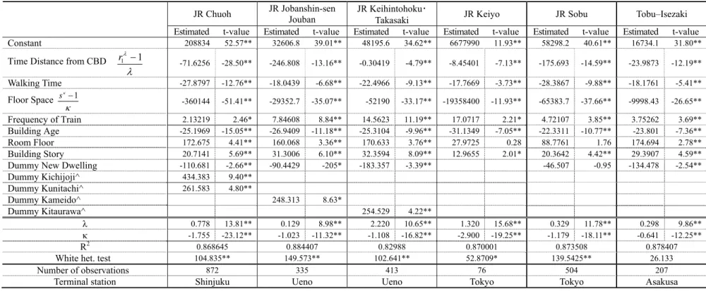
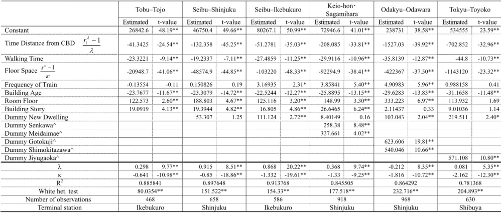
The estimation results for each rail line are shown in Tables 1-a and 1-b.

14 We also use frequency as an inverse indicator of average waiting time at the station in the estimation.

Table 1-a. Coefficient estimates of the rent function

JR Chuoh JR Jobanshin-sen Jouban

JR Keihintohoku^･

Takasaki ^{JR Keiyo JR Sobu} Tobu–Isezaki

Estimated t-value Estimated t-value Estimated t-value Estimated t-value Estimated t-value Estimated t-value Constant 208834 52.57** 32606.8 39.01** 48195.6 34.62** 6677990 11.93** 58298.2 40.61** 16734.1 31.80** Time Distance from CBD

λ

λ ₁

1 −

r -71.6256 -28.50** -246.808 -13.16** -0.30419 -4.79** -8.45401 -7.13** -175.693 -14.59** -23.9873 -12.19**

Walking Time -27.8797 -12.76** -18.0439 -6.68** -22.4966 -9.13** -17.7669 -3.73** -28.3867 -9.88** -18.1761 -5.41** Floor Space

κ

κ₋₁

s -360144 -51.41** -29352.7 -35.07** -52190 -33.17** -19358400 -11.93** -65383.7 -37.66** -9998.43 -26.65**

Frequency of Train 2.13219 2.46* 7.84608 8.84** 14.5623 11.19** 17.0717 2.21* 4.72107 3.85** 3.75262 3.69** Building Age -25.1969 -15.05** -26.9409 -11.18** -25.3104 -9.96** -31.1349 -7.05** -22.3311 -10.77** -23.801 -7.36**

Room Floor 172.675 4.41** 160.068 3.36** 170.633 3.76** 27.9725 0.28 88.7761 1.76 174.694 2.78**

Building Story 20.7141 5.69** 31.3006 6.10** 32.3594 8.09** 12.9655 2.01* 20.3642 4.42** 29.3907 4.59**

Dummy New Dwelling -110.681 -2.66** -90.4429 -205* -183.357 -3.39** -46.507 -0.95 -134.478 -2.54**

Dummy Kichijoji^ 434.383 9.40**

Dummy Kunitachi^ 261.583 4.80**

Dummy Kameido^ 248.313 8.63*

Dummy Kitaurawa^ 254.529 4.22**

Ȝ ^{0.778 13.81** 0.129 8.98** 2.220 10.65**} 1.320 15.68** 0.329 11.78** 0.298 9.86** ț ^{-1.755 -23.12** -1.023 -11.32** -1.108 -16.82**} -2.900 -19.25** -1.179 -18.11** -0.641 -12.25**

R² 0.868645 0.884407 0.82988 0.870001 0.873508 0.878407

White het. test 104.835** 149.573** 102.641** 52.8709* 139.5425** 26.133

Number of observations 872 335 413 76 504 207

Terminal station Shinjuku Ueno Ueno Tokyo Tokyo Asakusa

^ denotes particular station dummy.

* indicates significant at 5% and ** indicates significant at 1%.

Table 1-b Coefficient estimates of the rent function Tobu–Tojo Seibu–Shinjuku Seibu–Ikebukuro ^Keio-hon･

Sagamihara Odakyu–Odawara Tokyu–Toyoko Estimated t-value Estimated t-value Estimated t-value Estimated t-value Estimated t-value Estimated t-value Constant 26842.6 48.19** 46750.4 49.66** 80267.1 50.99** 72946.6 41.01** 238731 38.58** 534555 23.59** Time Distance from CBD

λ

λ ₁

1 −

r -41.3425 -24.54** -132.358 -45.25** -51.2781 -35.03** -208.085 -33.81** -1527.03 -39.92** -702.852 -32.96**

Walking Time -23.3221 -9.14** -19.2337 -7.11** -27.4859 -11.25** -29.9116 -10.96** -35.8139 -12.87** -44.8 -10.73** Floor Space

κ

κ₋₁

s -20948.7 -41.06** -48574.9 -44.85** -103220 -48.33** -92294.9 -38.41** -422367 -37.50** -1143120 -23.32**

Frequency of Train -0.13554 -0.11 0.150826 0.19 3.16935 2.31* 3.85841 5.40** 4.90983 5.96** 0.988158 0.41 Building Age -23.7677 -11.67** -23.3079 -14.72** -22.5244 -12.27** -25.8895 -13.15** -29.6283 -13.83** -31.1658 -11.48**

Room Floor 122.573 2.60** 188.803 4.67** 125.116 3.20** 148.99 3.30** 333.223 6.97** 113.932 1.69

Building Story 19.0919 4.13** 19.3944 4.82** 16.805 4.86** 26.6465 6.24** 2.11437 0.33 9.01036 1.14

Dummy New Dwelling 53.307 1.25 111.124 2.72** 8.40149 0.16 103.043 2.04** 219.511 2.40*

Dummy Senkawa^ 258.38 8.48**

Dummy Meidaimae^ 327.661 4.02**

Dummy Gotokuji^ 623.606 19.81**

Dummy Shimokitazawa^ 540.046 10.66**

Dummy Jiyugaoka^ 571.108 10.80**

Ȝ ^{0.298 9.77** 0.915 8.51** 0.868 20.22** 0.368 9.74** -0.212 8.35** 0.081 5.35**} ț ^{-0.641 -10.98** -0.85 -18.86** -1.332 -19.61** -1.33 -9.25** -1.816 -10.72** -2.162 -12.30**}

R² 0.885841 0.897648 0.913768 0.845505 0.864292 0.781368

White het. test 80.0354** 151.522** 154.33** 177.518** 232.716** 204.893**

Number of observations 468 658 586 918 968 630

Terminal station Ikebukuro Shinjuku Ikebukuro Shinjuku Shinjuku Shibuya

^ denotes particular station dummy.

* indicates significant at 5% and ** indicates significant at 1%.

Almost all explanatory variables are significant, and their coefficients are consistent with

theory in each equation, although dummy variables are also used. Rent decreases as the

distance from the CBD increases and as walking distance increases. An increase in the

frequency of trains increases the benefits and convenience of using rail because it reduces

the average waiting time. Thus, it raises rent. An increase in the age of a dwelling implies a

decline in housing quality, and lowers rent.¹⁵ Floor space has a positive coefficient, which

suggests that scale economies affect the market for rental housing. Both the dwelling floor

space and building story have positive and significant coefficients in almost all equations.

These suggest that taller buildings and dwellings on higher floors are generally of higher

quality.

Estimation of commuting cost

Next, we estimate unit commuting costs. The rent gradient (-R') is calculated from

the results in Tables 1-a and 1-b. We require data on s(r). Average floor space among

families living in residential districts around the stations was obtained from the 1995

census. We used data on floor space in Tokyo, which are aggregated by towns with stations.

However, these data are not available for prefectures other than Tokyo. Hence, for these

15 We use dummy variables of zero for new buildings and variables for the age of the dwelling, considering the possibility of non-linearity between the housing rent and age. In Japan, because there is little transaction volume in the secondary market for housing, a new building is valued more than an old building. See Yamazaki [23].

prefectures, we used average values for municipal districts.

Substituting the rent gradient and the floor space into equation (7), denoted by R'

and s(r), respectively, we calculate commuting costs between stations. Since data on

distance from the CBD are discrete for stations rather than continuous, as in equation (7),

the right-hand-side of equation (9) must be modified to incorporate the discrete term for

distance, ^Δr, which denotes time between stations.

That is:

( ) ^r ( ) ^{a r s} ( ) ^{r r}

s

r

R

c _{= −} ' ( ) _{≈ −}

_Δ

Using data obtained from equation (9) as the dependent variable, the following equation is

estimated:

δ

α

μ α

α

α +

⁻ + + Δ +

= ^{g r t}

c

¹

where

^{( )}

K r

g _≡ N and _δ is an error term.

However, there are insufficient observations for one region along one route, because

the available sample size is constrained by the number of stations within a distance of one

hour. There are only around 15 observations for the Seibu–Ikebukuro line. Pooling the data

for each region yields a sample size of 325 from which to estimate a commuting-cost

function of the congestion rate g, the time distance r and the pecuniary cost (the fare per

mile ^Δt).

The congestion rate is calculated by dividing the number of commuting ticket users

N(r) by the transportation capacity K in two hours at peak time.¹⁶ This marginal out-of-

pocket cost of commuting is defined as the difference between the monthly commuting

ticket fare from the CBD to the station and the fare to the previous station from the CBD.

We used a Box–Cox transformation of the congestion rate to account for possible non-

linearity because the variable appears to have an increasing effect on the marginal

disutility.¹⁷

Considering the interdependency between the congestion rate and the congestion

cost, we use the instrumental variables of the highest price in commercial area around each

station and the number of commuters from each station. The Hausman test rejects the

hypothesis about the endogeneity of these instrumental variables at 5% significance level.

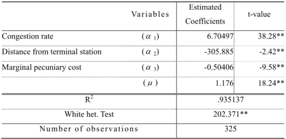
Estimation results for equation (9) are reported in Table 2.

16 The number of commuters and railroad capacity are available from the Institution for Transport Policy Studies [11].

17 We use the White test to detect heteroscedsticity. The White het test in Table 2 shows to reject a possibility of heteroscedsticity.

Table 2 Coefficient estimates of congestion cost

Va r i a b l e s ^Estimated

Coefficients ^t-value

Congestion rate (_α1) 6.70497 38.28**

Distance from terminal station (_α2) -305.885 -2.42** Marginal pecuniary cost (_α3) -0.50406 -9.58**

(_μ) 1.176 18.24**

R² .935137

White het. Test 202.371**

N u m b e r o f o b s e r v a t i o n s 325

**indicates significant at 1%, *indicates significant at 5%.

The positive and significant estimates for _α1and μ indicate that congestion generates

negative external effects on commuters. The negative and significant coefficient on

distance indicates decreasing marginal costs relating to distance, which suggests scale

economies affect journeys to work. The coefficient of the commuting fare _α 3 is negative

and significant. This seems somewhat a surprising result, because almost all commuters

are able to receive commuting allowances from firms. Furthermore, commuting costs paid

by firms can be deducted from profits.¹⁸ It implies subsidy to commuters.¹⁹ The

congestion cost is calculated from the empirical results obtained above. The congestion

charge must equal the increase in the commuting costs of other passengers induced by an

18 See Hatta and Ohkawara [5].

19 This result might show that 50% of passengers only get such implicit subsidy.

additional passenger. Since an increase in the number of passengers affects all passengers,

we calculate the extent to which an additional passenger imposes external effects on other

passengers.

We determine the marginal congestion cost as follows:

Marginal Congestion Cost N N

c

∂^∂

= ⁽¹¹⁾

g

g N c dN dg g c

∂^∂

=

×

∂^∂ ×

=

μ

μ

_α

α

= ⁻

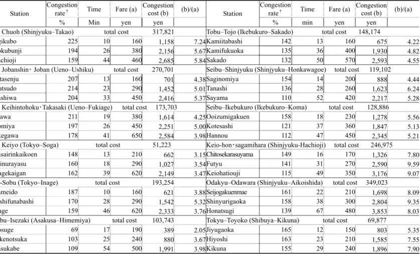
Using the estimates of _α1 and _μ in Table 2, we calculate estimated congestion costs

between the stations on each route. These estimates are reported in Table 3.

The congestion cost from the terminal station is the accumulated sum of the

congestion cost to the next station evaluated from the corresponding congestion rate in

each section. The congestion costs are between 2.05 and 9.59 times the regular fare, and as

expected, rise with the congestion rate. A decrease in the congestion rate in a particular

section reduces congestion costs in that section.

The congestion costs for the JR Keiyo line and the Tobu–Isezaki line seem relatively

low, while those for the Keio–Honsen , the Odakyu–Odawara and the Tokyu-

Toyoko lines are high. This is partly because the congestion rate for the Tobu–Isezaki line

is lower than on the other lines. On the other hand, since the fare on the JR Keiyo line is

higher than on the other lines, the ratio of congestion costs to fares appears lower than on

other lines. Appendix shows the average fares per time and distance for each line. The

Keio-honsagamihara, the Odakyu-Odawara and the Tokyu-Toyoko are cheaper and have

trains run more frequently than other lines. Their price policy partly explains higher ratio

of congestion cost to fares than other lines.

There are problems involved in examining why congestion costs differ between rail

routes. Since definitions of transportation capacity (K) differ between rail companies, so

do congestion rates and congestion costs. In addition, the ratios of commuting ticket users

to the total number of passengers at congested times also differ between rail routes.

Therefore, we must consider these issues when comparing charges between routes.

Table 3 Simulation results: congestion cost (units: total cost = million yen) Congestion

rate^{† Time Fare (a)}

Congestion cost (b) ^(b)/(a)

Congestion

rate^{† Time Fare (a)}

Congestion cost (b) ^(b)/(a) Station

% Min yen yen

Station

% min yen yen JR Chuoh (Shinjyuku–Takao) total cost 317,821 Tobu–Tojo (Ikebukuro–Sakado) total cost 148,174

Ogikubo 225 10 160 _1,158 7.24 Kamiitabashi 142 ^{13 160} 675 4.22

Kokubunji 194 26 380 _2,156 5.67 Kamifukuoka 135 ^{36 400} 1,930 4.82

Hachioji 159 44 460 2,685 5.84 Sakado 132 50 570 2,593 4.55

JR Jobanshin^･ Joban (Ueno–Ushiku) total cost 270,701 Seibu–Shinjyuku (Shinjyuku–Honkawagoe) total cost 119,102

Kitasenju 207 13 160 701 4.38 Saginomiya 154 14 200 888 4.44

Matsudo 214 23 290 _1,452 5.01 Tanashi 136 ^{28 260} 1,623 6.24

Kashiwa 204 33 450 2,416 5.37 Sayama 110 52 420 2,217 5.28

JR Keihintohoku^･Takasaki (Ueno–Fukiage) total cost 173,703 Seibu–Ikebukuro (Ikebukuro–Koma) total cost 128,886

Urawa 211 19 380 1,614 4.25Ooizumigakuen 158 18 230 1,278 5.56

Oomiya 197 26 450 2,251 5.00Kotesashi 121 37 360 1,847 5.13

Okegawa 178 41 650 2,584 3.98Hannou 112 47 450 2,345 5.21

JR Keiyo (Tokyo–Soga) total cost 51,223 Keio-hon^･sagamihara (Shinjyuku-Hachioji) total cost 246,975

Kasairinkaikoen 148 13 210 ₆₆₂ 3.15 Chitosekarasuyama 149 ^{16 170} 1,326 7.80

Shinurayasu 160 18 290 _1,027 3.54 Futyu 141 ^{31 270} 2,590 9.59

Inagekaigan 162 39 620 2,149 3.47 Keiohatiouji 115 49 350 3,176 9.07

JR-Sobu (Tokyo–Inage) total cost 193,254 Odakyu–Odawara (Shinjyuku–Aikoishida) total cost 349,023

Kameido 187 10 160 621 3.88 Seijogakuenmae 161 22 210 1,698 8.09

Nishifunabashi 170 28 290 _1,542 5.32 Shinyurigaoka 158 ^{38 300} 2,804 9.35

Inage 159 46 620 2,333 3.76 Honatsugi 139 67 480 3,853 8.03

Tobu–Isezaki (Asakusa–Himemiya) total cost 103,743 Tokyu–Toyoko (Shibuya–Kikuna) total cost 69,877

Kosuge 69 17 190 389 2.05 Jiyugaoka 165 12 150 803 5.35

Takenotsuka 103 25 240 880 3.67 Hiyoshi 163 23 210 1,585 7.55

Kasukabe 109 54 500 1,991 3.98 Kikuna 155 29 240 1,896 7.90

The congestion rate is a weighted average of congestion rates between stations, in which the weight is the ratio of the distance between stations to the total distance.

4. Conclusions

In this paper, we developed an econometric model for estimating congestion costs in

rail travel. Congestion charges have been estimated by using data obtained from the rent

functions for the railways in the Tokyo metropolitan area. An increase in congestion

generates an additional disutility that makes the rent gradient between stations steeper.

Thus, some of the difference between rents indicates the disutility due to congestion on the

train between stations. Paying attention to the rent gradient, in which the external effects of

congestion should be reflected, we included the congestion rate as an explanatory variable

in the estimation equation for the rent differential to the next station. We found that

congestion rates have a significant and positive effect on differences in rents. By using the

estimated coefficient of the congestion rate, we found that congestion charges are between

2.05 and 9.59 times the fares.

However, we cannot treat the estimated congestion cost as the optimal charge for the

following reason. We have not considered the rational reactions of consumers and firms to

the proposed congestion charges. Commuters would change their journey times if they had

to pay congestion charges at peak time. Some might commute to the CBD by car rather

than rail. Since the demand curve for rail travel is negatively sloped, our method

overestimates congestion costs, unless demand for rail services is inelastic.²⁰

However, in Japan, as Hatta and Ohkawara [5] pointed out, although commuters do

not directly bear commuting costs because they receive commuting allowances from firms,

they do experience time delays and fatigue when commuting. Thus, we may have

neglected the possibility of having overestimated congestion costs in the short run, since

we could not find the negatively sloped demand curve for commuter rail travel, as Table 2

shows. While our estimated congestion costs are optimal in short run, they are not optimal

in the long run, when firms can introduce flexible working hours and relocate to reduce the

commuting costs of workers.

We must examine how firms might seek to avoid congestion charges. Then, we

might find a negatively sloped demand curve for rail travel from which we could estimate

more accurately the optimal congestion cost, with the congestion externality being equal to

the congestion cost.

20 Another reason is due to the problem that the fare is not necessarily equal to the marginal cost of rail services because the fare is regulated by the authorities.

References

［₁］Arnott, R., de Palma, A. and Lindsey, R. “Economics of a Bottleneck” Journal of

Urban Economics, January 1990, vol.27, no.1, pp.111-30.

［₂］Arnott, R. J. and MacKinnon, J. G. “Market and Shadow Land Rents with

Congestion” American Economic Review, 1978. vol.68, no. 4, pp. 588-600.

［₃］Calfee, J. and Winston, C. “The Value of Automobile Travel Time: Implications for

Congestion Policy” Journal of Public Economics, 1998. vol.69, no.1, pp.83- 102.

［₄］Fujita, M. Urban Economic Theory, 1990. Cambridge University Press.

［₅］Hatta, T. and Ohkawara, T. “Housing and Journeys to Work in the Tokyo

Metropolitan Area,” in Y. Noguchi and J.M. Poterba (eds). Housing Markets in the United

States and Japan, 1991. University of Chicago Press, pp. 87-131.

［₆］Hatta, T. “On the Overcrowded Commuting in the Tokyo Metropolitan Area” in T.

Hatta and N. Yashiro (eds). Economic Solutions to Tokyo’s Problems, 1995. University of

Tokyo Press, pp. 59-90 (in Japanese).

［₇］Hatta, T. and Yamaga, H. “Fatigue Cost of Commuting and Optimum Congestion

Charge: An Empirical Estimation” 2001. Proceedings of the Annual Conference of the

Asian Real Estate Society in Japan.

［₈］Hayashiyama, Y. and N. Sakashita “Research on the Effect of Congestion Charges

on Congestion Easing” Highway and Automobile,1993. Express Highway Research

Foundation of Japan, vol.36, no.10, pp. 29-38 (in Japanese).

［₉］Henderson, J. V. Economic Theory and the Cities, Academic Press, 1977. New York.

Institution for Transport Policy Studies [2003] Toshi Koutsu Nenpo.

［₁₀］Kraus, M and Y. Yoshida "The Commuter's Time-of-Use Decision and Optimal

Pricing and Service in Urban Mass Transit, 2002. " Journal of Urban Economics”,

Vol.51, pp170-195

［₁₁］Mohring, H. Transportation Economics, 1976. Ballinger Publishing Company,

Cambridge, Mass.

［₁₂］Mohring H. “Congestion” in J. A. Gomez-Ibanez, W. B. Tye, C. Winston

(eds). Essays in Transportation Economics and Policy, 1999. The Brookings Institution,

Chapter 6.

［₁₃］Mun, Se-il “Peak-Load Pricing of a Bottleneck with Traffic Jams” Journal of

Urban Economics,1999. November 1999, vol.46, no.3, pp. 323-49.

［₁₄］Recruit Ltd. Shuukan Juutaku Jouhou; Shutoken (Metropolitan Area Version)

2002. November.

［₁₅］Shida K, A. Furukawa, T. Akamatsu, H. Ieda, “A Study of Transferability of

Parameters of Railway Commuter’s Disutility Function” 1989. Proceedings of

Infrastructure Planning, 12, The Infrastructure Planning Committee, pp. 519-525.

［₁₆］Small, K.A. “The Scheduling of Consumer Activities: Work Trips” American

Economic Review,1982. June 1982, vol.72, no. 3, pp. 467-79.

［₁₇］The National Land Agency White Paper on the Metropolitan Area 2003.

［₁₈］Vickrey, W. S. “Congestion Theory and Transport Investment” 1969. American

Economic Association, 59, pp. 251-260.

［₁₉］Yamauchi, H. “On the overcrowded commuting in Tokyo metropolitan Area” in T.

Hatta and N. Yashiro (eds). Economic Solutions to Tokyo’s Problems, 1995. University of

Tokyo Press. pp. 91-124. (in Japanese)

［₂₀］Yamazaki, F. An Economic Analysis of Land and Housing Markets in Japan, 1999.

University of Tokyo Press (in Japanese).

Appendix

Time Distance Fare Fare/Distance Fare/Time

Terminal

Station Edge Station (minute) (Km)

Number of

Station _(yen) Frequency (yen/km) (yen/minute)

JR Chuoh Shinjyuku Takao 51.6 42.8 22 540 55 12.6 10.5

JR Jobanshin^･

Joban Ueno Ushiku 55.1 52.8 22 950 40 18.0 17.2

JR

Keihintohoku^･

Takasaki Ueno Fukiage 57 54.2 12 950 50 17.5 16.7

JR Keiyo Tokyo Soga 46.3 43 17 740 25 17.2 16.0

JR Sobu Tokyo Soga 46.1 35.8 19 620 50 17.3 13.4

Tobu–Isezaki Asakusa Himemiya 52.5 38.4 28 500 70 13.0 9.5

Tobu–Tojo Ikebukuro Sakado 50.2 40.6 26 570 55 14.0 11.4

Seibu–

Shinjyuku Shinjyuku Honkawagoe 60.5 47.8 29 480 58 10.0 7.9

Seibu–

Ikebukuro Ikebukuro Koma 66 48.5 28 480 43 9.9 7.3

Keio-hon ^･

sagamihara Shinjyuku Hachioji 48.8 37.9 34 350 65 9.2 7.2

Odakyu–

Odawara Shinjyuku Aikoishida 66.2 48.5 35 520 61 10.7 7.9

Tokyu–

Toyoko Shibuya Kikuna 28.6 18.8 16 240 55 12.8 8.4