KIER DISCUSSION PAPER SERIES
KYOTO INSTITUTE
OF
ECONOMIC RESEARCH
KYOTO UNIVERSITY
KYOTO, JAPAN
Discussion Paper No.978
“Complementarity between Merit Goods and Private Consumption:
Evidence from estimated DSGE model for Japan”
Go Kotera
Saisuke Sakai
Complementarity between Merit Goods and Private Consumption:
Evidence from estimated DSGE model for Japan
Go Kotera
†Saisuke Sakai
‡September 2017
Abstract
This study constructs a dynamic stochastic general equilibrium model and empirically investigates
the effects of fiscal policy in Japan with focus on the functional difference in government
expenditures. Specifically, we divide government consumption into merit and public goods and
examine their external effect on private consumption. Our estimation using Japanese quarterly data
from 1981:Q1 to 2012:Q4 indicates that merit goods are complements for private consumption,
while public goods are substitutes, and consequently, the expenditure on merit goods has greater
positive effects on the economy than public goods. Furthermore, we show that Japanese government
expenditures are highly persistent and their response to the GDP gap and national debt accumulation
is limited. These findings suggest that the complementarity between private consumption and merit
goods is a major factor causing a fiscal crowding-in effect on private consumption.
JEL Classification: C11; E32; E62
Keywords: Edgeworth complementarity; Fiscal policy; DSGE modeling; Bayesian estimation
The views in this paper are the authors’ and do not necessarily represent those of the Ministry of Finance Japan and
the Policy Research Institute. We thank Ryokichi Chida, Kazuki Hiraga, Tatsuyoshi Matsumae, Koiti Yano, and the participants for the helpful comments and discussions at the 72nd General Meeting of the Japan Economic Policy Association and the 2015 Japanese Economic Association Autumn Meeting. In addition, we thank Taikei Araki, Takahiro Hattori, Hirokuni Iiboshi, Masahiko Nakazawa, Takefumi Yamazaki, and Yasutaka Yoneta for their helpful suggestions. Any remaining error is the sole responsibility of the authors.
†Corresponding author. E-mail: [email protected]. Policy Research Institute, Ministry of Finance Japan,
3-1-1 Kasumigaseki, Chiyoda-ku, Tokyo 100-8940, Japan.
1.
Introduction
In response to prolonged stagnation since the 1990s and its aging population, Japan increased its
government spending and as a result, the gross debt-to-GDP ratio has risen to more than 200 percent
as of 2017. These conditions warrant fiscal policies that are more efficient, and therefore, it is
imperative to investigate the effects of government spending. This study empirically examines the
effect of fiscal policy in Japan with focus on differences stemming from types of government
spending. More specifically, we construct a dynamic stochastic general equilibrium (DSGE) model
with two categories of government consumption, that is, merit goods and public goods, and
government investment and estimate their effects using Bayesian techniques.
Differences in the effects of government expenditures in a model can be attributed to two
channels. First is their non-wasteful properties. In terms of government investment, accumulated
social capital has a positive external effect on production (e.g., Baxter and King, 1993). Meanwhile,
the non-wasteful nature of government consumption is Edgeworth complementarity or
substitutability between public and private consumption. If they are complements (substitutes), an
increase in government consumption crowds in (out) private consumption and consequently,
enhances (diminishes) the positive effect on output. Therefore, the effect of government
consumption expenditure largely depends on whether the relationship is complementary or
substitutive. While some empirical studies such as Aschauer (1985) and Ahmed (1986) report
substitutability, Karras (1994), Evans and Karras (1996), and recent DSGE studies focusing on the
United States (Bouakez and Rebei, 2007; Fève et al., 2013) and the euro area (Coenen et al., 2013)
show complementarity. Similarly, studies on Japan suggest complementarity (Okubo, 2003; Iwata,
2013).
While the above-mentioned works focus on total government consumption, Fiorito and
consumption into two categories, merit and public goods, and investigate their individual
relationship with private consumption. While merit goods are represented by healthcare, education,
and social protection spending, which are rival in private consumption and affect welfare through
distribution policies, public goods comprise spending on general public services, defense, and so on
and are mostly non-rival in nature. Fiorito and Kollintzas (2004) demonstrate the complementarity of
merit goods and substitutability of public goods in 12 European countries.
The second factor causing the differing effects of government expenditure is policy rules. While
in most previous studies, fiscal policy rules include terms related to a lag, output gap, and
government debt, the specification is not uniform.1 However, the specification of spending rules
plays an important role in evaluating policy effects. Corsetti et al. (2012) point out the importance of
“spending reversals,” which indicate that government expenditure decreases with government debt
accumulation. Spending reversals reduce future inflation resulting from a government spending
shock and the rise in interest rate through the monetary policy rule, and therefore, increase the effect
of a fiscal expansion.2 Furthermore, Fève et al. (2013) show that an estimation without a
countercyclical output gap term in fiscal policy rules underestimates the degree of Edgeworth
complementarity. Previous studies, such as Lane (2003), Abbott and Jones (2011, 2012), and Frankel
et al. (2013), provide empirical evidence on the cyclicality of government spending in developed
countries as follows: (1) total government spending is countercyclical or acyclical and (2) certain
spending categories demonstrate procyclicality.
This study investigates the degree of complementarity or substitutability of merit goods and
1
For example, Bouakez and Rebei (2007), Galí et al. (2007), and Kato and Miyamoto (2013) adopt the simple first-order autoregressive rules. Iwata (2011) includes lag and output gap terms in the rules and in Iwata (2013), government expenditures respond to the previous ones and debt-to-GDP ratio. Coenen et al.’s (2013) policy rules comprise lag, output gap, debt-to-GDP ratio terms, and moving average of policy shocks.
2
public goods in Japan by conducting a Bayesian estimation using a DSGE model. In analyzing the
effect of fiscal policy in Japan, separating merit goods from public goods is crucial. As shown in Fig.
1, merit goods expenditure as a share of nominal GDP rapidly increased since the mid-2000s
because of the growth in healthcare and social protection spending. This growth possibly reflects the
rapid increase in the aging population and evaluating the effects of merit goods expenditure
contributes to the discussion on present and future policy design under severe fiscal conditions.3
Following the above-mentioned studies, we specify fiscal spending rules, including output gap and
debt-to-GDP ratio terms, and examine whether fiscal policy in Japan includes spending reversals and
if it is pro- or countercyclical.
[Fig. 1]
Additionally, our study is related to the well-known “puzzle” of the relationship between
government spending and private consumption. While standard dynamic general equilibrium models
predict the negative effect of government spending on private consumption, previous empirical
studies, such as Blanchard and Perotti (2002), show a positive one.4 Drawing on the literature, our
DSGE model includes the following four factors to overcome this puzzle: (1) productive social
capital (Baxter and King, 1993), (2) household under liquidity constraint (Galí et al., 2007), (3)
spending reversals rule of government spending (Corsetti et al., 2012), and (4) Edgeworth
complementarity between government spending and private consumption (Bouakez and Rebei,
2007; Ganelli and Tervala, 2009; Fève et al., 2013). This study, thus, provides some insight into
which of these factors contributes to the positive response of private consumption to government
3
Population estimates by the Statistics Bureau, Ministry of Internal Affairs and Communications, show that those aged 65 years and above as a share of total population increased from 17.5% to 23.2% during 2000–2010 (http://www.stat.go.jp/english/data/jinsui/2.htm).
4
spending shocks.
For the Bayesian estimation, we employ data from 1981:Q1 to 2012:Q4 and show that merit
goods are complements for private consumption, while public goods are substitutes. In addition, we
suggest that the degree of complementarity or substitutability largely affects the quantitative
evaluation of government spending. Further, we conduct a time-series analysis using a vector
autoregressive (VAR) model to support the quantitative difference in effects between merit and
public goods expenditure. However, the estimated complementarity should be carefully interpreted
because it possibly stems not from household preference but from the characteristics of Japan’s
national care system, under which people incur only a part of their health and long-term care costs
and the remaining is paid by government.5 In this case, the degree of complementarity can be
overestimated because an increase in private consumption partly involves additional expenditure on
merit goods. Therefore, we conduct several robustness checks for the complementarity. The results
confirm the complementarity, although the degree is smaller than that in the main result. Throughout
the analyses, the multipliers during 1981–2012 for expenditures on merit goods, public goods, and
government investment are approximately 1.75–1.91, 0.25–0.48, and 0.93, respectively. Furthermore,
we find that the behavior of government expenditures in Japan can be mostly explained by the inertia
and the influences of spending reversals and cyclicality are quantitatively small.
The remainder of this paper is organized as follows. Section 2 provides the empirical result for a
VAR model. Section 3 presents a DSGE model with Edgeworth complementarity (or substitutability)
between government and private consumption. Section 4 estimates a DSGE model using a Bayesian
technique and shows the result. Section 5 conducts robustness checks on the results, and Section 6
concludes.
5
2.
Time-series analysis
Preceding the analysis using a DSGE model, we perform a time-series analysis. To investigate
the effects on the basis of types of government spending, we individually consider government
consumption and investment and further divide government consumption into merit and public
goods. The VAR model includes the following ten variables: real GDP, real private consumption,
real private investment, hours worked, inflation rate, nominal interest rate, real wage, and three
government spending variables. These variables are common to the Bayesian estimation of the
DSGE model in Section 4.
2.1
. Data and Methodology
We employ the following quarterly data in Japan for 1981:Q1–2012:Q4. Data for nominal GDP,
nominal consumption, nominal investment, and nominal government expenditures are obtained from
the Cabinet Office. As for government consumption, we define merit goods expenditure as
individual consumption expenditure by the general government, most of which comprises spending
on healthcare, social protection, and education, and public goods expenditure as collective
consumption expenditure.6 Data for nominal wages and hours worked are obtained from the
monthly labor survey conducted by the Ministry of Health, Labour and Welfare, and inflation rate is
the log difference of the consumer price index (CPI) published by the Ministry of Internal Affairs
and Communications. As nominal interest rate, we use the unsecured overnight call rate available in
statistics by the Bank of Japan.7
GDP, consumption, investment, and three government expenditures are per worker terms, and
6
Collective consumption by the general government also includes spending on healthcare, education, and social protection (e.g., expenditures on R&D); however, their fractions in government collective consumption are considerably smaller than those in government individual consumption.
7
these six variables and wage are in logs and deflated by CPI. All series, except nominal interest rate,
are seasonally adjusted. In addition, all series are one-sided Hodrick–Prescott (HP) filtered because
the augmented Dickey–Fuller test and Phillips–Perron test suggest they have unit roots and the
impulse response analysis based on the present DSGE model (see Section 4) employs de-trended
variables.8
The Schwartz criterion suggests that the optimal number of lags in the VAR model is 1. To
identify the government spending shock, we adopt Cholesky decomposition and order each
government spending variable first, similar to previous works such as Bouakez and Rebei (2007),
Galí et al. (2007), and Kato and Miyamoto (2013). This implies that government spending shocks
are more exogenous and pre-determined than other variables.
2.2. Impulse responses
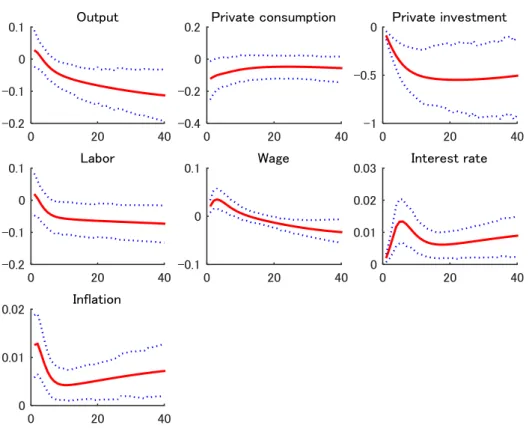
Figs. 2 and 3 illustrate the impulse responses of key variables to positive merit goods and public
goods expenditure shocks, respectively. The shapes of impulses are similar in both cases, and almost
all variables increase.
[Fig. 2]
[Fig. 3]
On the other hand, the significance tends to differ, and in particular, the effects of public goods
shock on output, private consumption, labor, and wage are more ambiguous than those of merit
goods shock. Therefore, the results suggest that the positive effect of merit goods spending on the
economy is larger than that of public goods spending. We do not present a figure for government
8
investment because the shapes of impulses are similar to those for positive merit goods and public
goods expenditure shocks and this study focuses on the difference between the effects of merit and
public goods.9
3.
Model
Our model is similar to Hirose and Kurozumi’s (2012) DSGE model, which is based on Smets
and Wouters (2007). We exclude investment-specific technology from their model and instead,
incorporate the following: (1) fiscal policy rules, (2) public capital that enhances the productivity of
intermediate goods producers, (3) non-Ricardian households under liquidity constraint, and (4)
Edgeworth complementarity (or substitutability) between the government and private consumption
of Ricardian households. More specifically, following Fiorito and Kollintzas (2004), we divide
government consumption into merit goods and public goods and introduce the effective consumption
of Ricardians that allows for non-separable government consumptions. Furthermore, similar to Erceg
et al. (2006), Hirose and Kurozumi (2012), and Iwata (2013), our model includes a balanced growth
trend.
3.1. Households
There is a continuum of infinitely lived households whose sum is unity. Households are divided
into two types: fraction − � is Ricardian households who can freely access financial markets and
optimize their intertemporal behavior, and the remaining are non-Ricardian households under
liquidity constraints.
The utility function of Ricardian household ℎ ∈ [�, ] is given by
9
� ∑ � ��{( �
� ℎ − �
�−� ℎ ) −�
− � − �
−� � � ℎ +�
+ � + � �� + �� ��� }
∞
�=
, (1)
where �� ℎ and � ℎ are the effective consumption and labor supply of Ricardian household
ℎ, respectively. � is the technology level following the non-stationary stochastic process
log �= log + log �− + � , where is the gross steady-state growth rate and � is a
technology shock. � and � are shocks to the discount factor ∈ , and labor supply,
respectively. � > denotes the inverse of the elasticity of the intertemporal substitution, � > is
the inverse of the elasticity of labor supply, and � ∈ , measures the degree of habit formation
in consumption. We define the effective consumption of Ricardian household ℎ as follows:
�� ℎ = �� ℎ + � �� + �����,
where �� ℎ is the private consumption of Ricardian household ℎ, and �� and ��� represent
two types of government consumption, merit goods and public goods. If , ∈ { , } is
negative (positive), the marginal utility of private consumption is increasing (decreasing) in
government consumption, implying complementarity (substitutability) between private and
government consumption.10 Functions � and �� in Eq. (1) satisfy �′ > and ��′ > ,
ensuring that the marginal utility of government consumption is positive.
The budget constraint of Ricardian household ℎ is given by
�� ℎ + ��� ℎ + �� ℎ = � ℎ � ℎ + � � ℎ ��−� ℎ + �−
� �−
� ℎ +
� ℎ − ��, (2)
where ��� ℎ is private investment, �� ℎ is government bonds, � ℎ is the capital utilization
rate, ��−� ℎ is the capital stock at the beginning of period , � ℎ is the dividend from
intermediate goods firms, and �� is the lump-sum tax levied on Ricardian households. �, � ℎ ,
�, and �− , respectively, denote the gross inflation rate of final goods price ��, real wage, gross
10
real rental rate of capital, and gross nominal return on the government bond. The first-order
conditions for �� ℎ and �� ℎ are given by
Λ�= �� ��− � �−� −�− ��� �+1� �+� − � �� −�,
�= ���+ � �+ ,
where Λ� is the Lagrangean multiplier. Index ℎ is omitted because all Ricardians face the same
decision-making problem regarding �� ℎ and �� ℎ in the presence of a complete insurance
market.
Under the monopolistic competition, households supply their differentiated labor services,
given the labor demand by intermediate goods firms. According to Galí et al. (2007), we assume that
intermediate goods firms uniformly demand differentiated labor services from both types of
households. Then, the demand for labor service ∈ [ , ] is expressed as
� = �
� −��
�. (3)
Here, � is the aggregate labor demand defined as an aggregation technology
�= ∫ � ��− ⁄��
��⁄��−
, where �� > is the elasticity of substitution across labor
services. � denotes the aggregate wage satisfying
�= ∫ � −��
−�� ⁄
. (4)
Ricardian households set their wage as per Calvo (1983); they have the opportunity to re-optimize
their wage with probability − in each period. Meanwhile, Ricardians cannot set an optimal
wage with probability and then, choose their nominal wage on the basis of both gross
steady-state growth rate and a weighted average of past and steady-state inflation. Specifically,
unoptimized nominal wage rule is denoted by
where is the steady-state inflation rate and ∈ [ , ] is the relative weight on past inflation.
The optimal wage is chosen to maximize
��∑ [Λ�+ �+ ℎ � ℎ ∏ { �+ − �
�+ − } =
− �+
�
�+ �+−� �+ ℎ +�
+ � ]
∞
=
subject to Eq. (3). Representing the optimal wage as �∗, the first-order condition for � ℎ is
��∑ Λ�+ �+
�+ [
�∗ �+ ∏ {
��+ −1 � � � ��+ } = ] −1+��+ ��+ {
�∗∏ { ��+ −1�
� � ��+ } = ∞ = − ( + �+ ) �+� �+ �+−� Λ�+ ( �+ [ � ∗ �+ ∏ { ��+ −1
� � � ��+ } = ] −1+��+ ��+ ) � } = ,
where � ≡ / �� − denotes the wage markup. Moreover, we assume that non-Ricardian
households earn aggregate wage in each period.11 Then, Eq. (4) can be expressed as
�−�� = −
(
�∗ −�� + ∑ [ �−∗ ∏ { ��−�
� �
��− +1} = ] −�� ∞ = ) .
Ricardian household ℎ optimally chooses � ℎ , ��� ℎ , and ��� ℎ under Eq. (2) and the
following law of motion of capital stock:
��� ℎ = − ( � ℎ ) ��−� ℎ + − ( ��
� ℎ
��−� ℎ �
) ��� ℎ , (5)
where function denotes the depreciation rate of capital and satisfies ′> , ′′> , =
∈ , , and ′ ⁄ ′′ = . Thus, higher utilization further depreciates capital stock. Function
represents the adjustment cost of investment and is given by = − / � . � denotes
a shock to the adjustment cost of investment. The first-order conditions for � ℎ , ��� ℎ , and
11
��� ℎ are given by
� = � ′ � ,
= �{ − (�� �
��−� �
) − ′(���
��−� �
)����
�−� �
} + ��ΛΛ�+
� �+
′(��+�
��� �+1
) ��+��
��
�+1
,
�= ��ΛΛ�+
� { �+ �+ + �+ ( − �+ )}.
Here, � is defined as �≡ Λ�/Λ�, where Λ� is the Lagrangean multiplier with respect to Eq. (5).
Index ℎ can be omitted since decisions for � ℎ , ��� ℎ , and ��� ℎ are common to all Ricardian
households.
Fraction � of households includes non-Ricardian households who are under liquidity
constraints and do not possess any asset. The budget constraint of a non-Ricardian household is
denoted by
���= � �− ���,
where ��� and ��� denote private consumption and lump-sum tax. As noted above, all
non-Ricardians earn the aggregate wage and supply labor services equal to aggregate labor. It
follows that they obtain equal disposable income and consume it all. As a result, non-Ricardian
households can be regarded as homogenous rule-of-thumb consumers. The greater the number of
non-Ricardian households, the larger the impact of fiscal expansion because unlike Ricardian
households, they consume all of the increment in disposable income. For simplicity, we assume that
lump-sum tax is evenly levied on both households, that is, �� = ���= �.
3.2. Firms
A final goods firm in the perfectly competitive market produces a final good with the following
�= ∫ � ���−
���
��� ���−
,
where � is a final good available for consumption and investment; � is an intermediate good
produced by the intermediate goods firm , which is continuously and uniformly distributed on
[ , ]; and ��� > is the elasticity of substitution across intermediate goods. Given the intermediate
goods price �� , the demand function for � is derived as
� = ���
� −���
� (6)
and the relationship between the final goods price and intermediate goods prices is then represented
by
= (∫ (���
� )
−���
) −��
�
. (7)
Each monopolistically competitive intermediate goods firm has the following production
function:
� = �−�−�( ���− )�� −�(��−� )�− Φ �, (8)
where ∈ , , > , and + < . ��−� is public capital at the beginning of period , and
Φ > represents fixed cost. This specification is employed in numerous previous studies, such as
Baxter and King (1993) and Iwata (2013); implies there are constant returns to scale in privately
provided factors; and is the positive externality of the public capital. This productivity-enhancing
property increases the effectiveness of government investment through the accumulation of public
capital.
Cost minimization for intermediate goods firms leads to the following condition:
�= { − �
�} −�
� � ��−� �
−�
,
intermediate goods firm. Index is omitted since all firms face the same problem. Furthermore,
using Eqs. (6) and (8) and first-order conditions for cost minimization, we obtain the aggregate
output as follows:
�∫ ��� �
−���
= �−�−� ���− � � −�(��−� )�− Φ �,
where ��− ≡ ∫ ��− and �≡ ∫ � .
Intermediate goods firms follow the Calvo price-setting rule. While intermediate goods firms
can optimize their price with probability − � in each period, they set their price according to the
following rule:
�� = �−�
� −��
��− ,
with probability �. Parameter �∈ [ , ] represents the relative weight on the previous inflation
rate. The optimal price is chosen to maximize
��∑ � ΛΛ�+
� [ �� ��+ ∏ { �+ − �� } = − �+ ] �+ ∞ =
subject to Eq. (6). Representing the optimal price as ��∗, the first-order condition for �� is
��∑ � ΛΛ�+
� �+� [
��∗
��∏ { ��+ −1
� �� � ��+ } = ] −1+��+ � ��+� �+ [�� ∗ ��∏ { ��+ −1
� �� � ��+ } = ∞ = − ( + �+� ) �+ ] = ,
where ��≡ / ���− denotes the price markup. Then, Eq. (7) can be written as
3.3. Monetary and fiscal authorities
Monetary policy is implemented according to the following standard rule:
log � = ��log �− + − �� {log + ��� 4 ∑ log �−
=
+ ��log � �∗} + �
�,
where is the gross nominal interest rate in the steady state and �� denotes a monetary policy
shock. �∗ denotes potential output and is defined as
�∗ = �−�−� �− � −� � �− �− Φ �,
where and represent the steady-state values of the capital utilization rate and labor. and �
are steady-state values of de-trended private capital ��/ � and de-trended social capital ���/
�, respectively.
We consider two types of government consumption, merit goods and public goods, and
government investment. They are financed by government bonds and lump-sum tax levied on
households. The government budget constraint is then
�= �−
� �− + �� + �� �+ �
�− �,
where � is the aggregate government bond and �� is government investment. Social capital is
accumulated by government investment as follows:
��� = − � �
�−� + ��,
where g is the depreciation rate of social capital.
Fiscal policy rules are defined by
log �� = �� log ��− + log + − �� log � + �� log �−
�−∗ + �
� log �− / �− � �
+ �� ,
log ��� = ���(log �
�−� + log ) + − ��� log � �+ ���log �− �−∗ + �
��log �− / �− � �
log �� = ��(log ��− + log ) + ( − ��) log � + �� log �− �−∗ + �
� log �− / �−
� � + ��,
where , ∈ { , , } denotes the steady-state values of ��/ � and � � is the target share of
government bond in aggregate output. �, ∈ { , , } are shocks to each fiscal policy. In our
model, government spending rules include a smoothing term and respond to output gap and the
deviation of the debt-to-output ratio from its target in the previous period. As pointed out by Fève et
al. (2013), an estimation without a countercyclical component underestimates the effect of
Edgeworth complementarity and consequently, the fiscal multiplier. The positive (negative) sign of
� , ∈ { , , } denotes the procyclicality (countercyclicality) of government spending.
Moreover, if � < , ∈ { , , }, government expenditure decreases in response to an
increase in government debt. Such “spending reversals” rules (Corsetti et al., 2012) reduce future
inflation by government spending shocks and a rise in interest rate through the monetary policy rule.
This mechanism induces an increase in private consumption.
The taxation rule is denoted by
log �= �� log �− + log + − �� log �� − ��log �−
�−∗ − �
�log �− / �−
� � ,
where � represents a steady-state value for �/ �. Analogous to fiscal policy rules, lump-sum tax
depends on its own lagged value, output gap, and debt-to-output ratio.
3.4. Market clearing, aggregation, and structural shocks
The market clearing condition is denoted by
� = �+ ��+ �� + ���+ ��+ � �.
Here, � and �� are aggregate consumption and aggregate investment satisfying
�= � ���+ ∫ �� ℎ ℎ
� ,
��= ∫ ��� ℎ ℎ
denotes the other de-trended demand factor, such as net exports at a steady state, and � is the
exogenous demand shock. Private capital and government bond are aggregated as follows:
��= ∫ ��� ℎ ℎ
� ,
� = ∫ �� ℎ ℎ
� .
Finally, each structural shock follows a first-order autoregressive process with an i.i.d.- normal error
term:
� = �− + ��, ��~�( , � ),
where ∈ { , , , , , , , , }.
As noted above, our model contains a balanced growth trend. Specifically, ��, ���, ��, �,
���, ��, ���, ��, ���, �, �∗, ��, �, �� , ���, ��, �, �, and �∗ increase at gross rate on
the balanced growth path. In estimating the model parameters, we de-trend and log-linearize the
model. The de-trended and log-linearized model is presented in Appendix.
4.
Bayesian estimation
The model parameters are estimated with a standard Bayesian technique based on the Markov
Chain Monte Carlo (MCMC) method. Using the solution equations of the log-linearized model and
observation equations linking the model variables to data, we can evaluate the log likelihood
function using the Kalman filter. Furthermore, combining the log likelihood with the prior
distribution of parameters, we perform MCMC sampling on the basis of a Metropolis–Hastings
algorithm to obtain the posterior distribution. We generate two Markov chains with 500,000 draws
4.1. Data, calibration, and priors
Most studies on Japanese DSGE models with Bayesian estimations adopt data prior to 1999 to
exclude the zero interest rate periods (e.g., Sugo and Ueda, 2008; Iwata, 2011, 2013; Hirose and
Kurozumi, 2012). A zero lower bound (ZLB) constraint for interest rate faces problems of
non-linearity and indeterminacy (e.g., Braun and Waki, 2006). Furthermore, a Bayesian estimation
based on a Kalman filter cannot be applied to non-linear models.12 Meanwhile, conducting a Monte
Carlo simulation, Hirose and Inoue (2016) show that an estimation neglecting the ZLB constraint
has limited effects on posterior mean estimates and impulse responses. Therefore, we use a dataset
with more recent information and estimate the model using data prior to 1999 in the robustness
analysis.
We employ ten quarterly data series in Japan from 1981:Q1 to 2012:Q4, as follows: real GDP,
real private consumption, real private investment, real wage, real merit goods consumption, real
public goods consumption, real government investment, labor hour, inflation rate, and nominal
interest rate.13 These series are related to model variables through the following observation
equations: [ Δln � Δln � Δln�� Δln � Δln��
Δln��� Δln��
ln�
Δln��
ln � ]
= [ ∗+ � ∗+ � ∗+ � ∗+ � ∗+ � ∗+ � ∗+ � ∗ ∗+ ∗] + [ ̃�− ̃�− ̃ �− ̃�− �̃�− �̃�− ̃�− ̃�− ̃� − ̃�− ̃��− ̃�−� ̃�− ̃�− ̃� ̃� ̃ � ] , 12
Kitamura (2010) employs a particle filter technique and estimates a DSGE model considering the ZLB constraint.
13
where lower-case letters with tildes denote the log-deviation of de-trended variables from their
steady-state level; ∗, ∗, and ∗ are the net growth rate of technology, net inflation rate, and net
real interest rate at steady state, respectively; and is the steady-state level of labor hour.
Following Sugo and Ueda (2008) and Hirose and Kurozumi (2012), certain parameters and
steady-state values are calibrated as follows. The capital elasticity of output and the steady-state
depreciation rate of capital are set at 0.37 and 0.015. The output ratios of merit goods
consumption / , public goods consumption �/ , and government investment / are 0.083,
0.067, and 0.05, respectively.14 The target debt-to-output ratio � �, output ratio of external demand
at steady state / , and depreciation rate of social capital � are set at 0.6, 0.1, and 0.01,
respectively.
While the priors of most estimated parameters are selected on the basis of previous works on
Japan, such as Sugo and Ueda (2008), Hirose and Kurozumi (2012), and Iwata (2013), we adopt the
following priors regarding the parameters of our interest. To neutrally evaluate the degree of
Edgeworth complementarity or substitutability, the priors of � and �� are normal distributions
with mean 0 and standard deviation 1.5. While Fève et al. (2013) show that the cyclicality of
government spending affects the estimation of complementarity parameters, to the best of our
knowledge, there is no consensus on whether each government spending rule in Japan is
countercyclical or procyclical. Therefore, we choose normal distributions with mean 0 and standard
deviation 0.5 as priors of �� , ���, and �� . Moreover, to investigate whether the spending
reversals effect of government expenditures are observed, �� , ���, and �� are ex ante assumed
to follow normal distributions with mean 0 and standard deviation 0.5. Finally, unlike previous
studies, we estimate the parameter of wage markup and choose a normal distribution with mean
0.2 and standard deviation 0.1 as the prior.
14
4.2. Posterior distributions
Table 1 presents the priors, posterior means, and 90% credible intervals. Most of the posterior
means of the standard structural parameters are similar to those of previous studies that do not
account for zero interest rate periods. The estimated posterior means of � and �� are −1.62
and 0.9, respectively. These results indicate that merit goods are complements for private
consumption, while public goods are substitutes, similar to Fiorito and Kollintzas (2004) who focus
on European countries. The posterior mean of is 0.11, which is larger than Iwata’s (2013) result.
The estimated mean value of the fraction of non-Ricardian households � is 0.08, which is
considerably smaller than that in Iwata (2011).15
[Table 1]
Our estimation indicates that all government spending in Japan are highly persistent and
fluctuate not by GDP gap and debt-GDP ratio but by shocks because the posterior means of �� ,
���, and �� are, respectively, 0.98, 0.97, and 0.96. The estimated posterior means of �� , ���,
and �� are 0.4, 0.36, and −0.02, respectively, indicating that government consumption and
investment are weakly procyclical and countercyclical, respectively. According to Fève et al. (2013),
the estimated relationship between government and private consumption are more likely to be
substitutive under a procyclical spending rule. However, the influence of the procyclicality of
government spending on the estimation of complementarity parameters is considered to be negligible
because, as shown above, the coefficients of lag variables are sufficiently large and the 90% credible
intervals of coefficients for output gap terms include zero in all cases. The posterior means of
15
�� , ���, and �� are, respectively, −0.19, −0.07, and 0.18, and the spending reversals effect is
significantly observed only in merit goods. Similar to the result for GDP gap terms, the spending
reversals effects have a limited impact on the effect of fiscal expansion given the strong inertia in
spending rules.
4.3. Impulse responses and fiscal multipliers
Figs. 4 and 5 present the impulse responses of key economic variables to merit goods and
public goods expenditure shocks. Private consumption increases in response to a merit goods shock
and slightly decreases to a public goods shock. This opposite response stems from the degree of
complementarity of merit goods and public goods because both estimated spending rules, and
therefore, their spending streams generated by shocks are almost the same. This result does not
completely replicate that of the above VAR analysis because the impulse responses in Section 2
show that both merit and public goods shocks significantly increase private consumption.
Meanwhile, both analyses suggest that a merit goods shock has a more positive effect on private
consumption than a public goods one.
Furthermore, although Galí et al.’s (2007) numerical analysis shows that the fraction of
non-Ricardian households ω is required to be roughly 0.25 to induce the crowding-in of private
consumption by fiscal expansion in the case where the rule-of-thumb household is the only source of
crowding-in, our result indicates that crowding-in arises through Edgeworth complementarity even if
ω = 0.08. This suggests that the complementarity between private and government consumption is
quantitatively a significant factor in explaining the crowding-in of private consumption.
[Fig. 4]
[Fig. 5]
of a public goods shock are more ambiguous than those of merit goods, particularly on output and
labor. These trends are similar to those of time series analysis results.
The fiscal multipliers for merit goods and public goods are 1.91 and 0.26, reflecting the
estimates of complementarity parameters. This result indicates that the effect of fiscal expansion
largely varies by type of fiscal spending and merit goods expenditure has a large positive effect on
the economy. The fiscal multiplier for public investment is 0.92, which is similar to the multiplier
reported in previous studies.
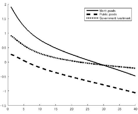
Next, we examine the medium- and long-term effects of government expenditures. Fig. 6
depicts the present-value multipliers defined by Mountford and Uhlig (2009). The effect of both
government consumptions monotonically decreases and has a negative impact in the medium and
long run. In particular, the effect of public goods expenditure is negative in approximately the fourth
period and the cumulative negative impact is maintained in the long run. On the other hand, the
government investment maintains a positive effect in the long run through the positive external
effect of social capital.
[Fig. 6]
5.
Robustness checks
This section conducts a robustness analysis and scrutinizes the complementarity between merit
goods and private consumption found in the previous section. Specifically, we estimate models with
certain alternative specifications and different datasets and then, compare the results.
5.1. Alternative specifications
We now estimate the model on the basis of the two following alternative specifications. First, as
consumption can stem from Japan’s national care system, in which people incur only a part of their
health and long-term care payments, rather than household preferences. In this case, the
complementarity between merit goods and private consumption can be overestimated. To consider
this institutional effect, we modify the observation equation of merit goods as follows:
Δln�� = ∗+ � + ̃� − ̃�− + �� ∗+ � + ̃�− ̃�− , (9)
where �� > . This equation exhibits that the observed variation in merit goods expenditure is
partially associated with that in private consumption.
Second, we assume that the complementarity parameters regarding merit and public goods are
common, that is, � = ��. This specification assumes a situation in which merit and public
goods are not distinguished as in Okubo (2003) and Iwata (2013).16 We then show how the division
of government consumption affects the estimation result and discuss the validity of specifications.
Table 2 presents the estimation results for the selected parameters under alternative
specifications and in the baseline model presented in the previous section. Column 1 presents the
result for the case in which the observation equation for merit goods expenditure is replaced by Eq.
(9) and the absolute value of the posterior mean of � is smaller than that in the baseline model.
This indicates that the complementarity between merit goods and private consumption is weaker and
as a result, the multiplier for merit goods is smaller. Meanwhile, since the log data density in the
baseline model is greater than that in the model with Eq. (9), the degree of complementarity in the
baseline may not be necessarily overestimated.17 The estimation results of the other parameters are
almost the same as those in the baseline model, except for ��. ��, the degree of substitutability
16 Note that the policy rules differ between merit and public goods, which is similar to the above analysis. Therefore,
the difference in the effects of merit and public goods in this model can be attributed to their policy rules.
17
between public goods and private consumption, is estimated to be smaller. Therefore, the multiplier
for public goods increases.
[Table 2]
Column 2 presents the estimation results in the case where complementarity parameters are
common to merit and public goods. The posterior mean of � is −0.47, indicating that government
consumption is a complement of private consumption and the degree is smaller than that of merit
goods in the baseline model. This result is almost the same as Iwata’s (2013) estimates and suggests
that the complementarity of merit goods is partially offset by the substitutability of public goods and,
consequently, total government consumption seems to be weakly complemented with private
consumption. Moreover, in this specification, the log data density is smaller than that in the baseline
model, and thus, the baseline specification can better explain the data series.
5.2. Different datasets
In this subsection, we estimate our model using two datasets. First, we limit the sample period
to 1998:Q4. From 1999 to 2012, Japan experienced a rapid increase in its aging population and in
2000, it launched the public long-term care insurance system. These events have induced an increase
in health and long-term care payments by households, and consequently, in merit goods expenditure
through the systems. In this case, complementarity can be overestimated because spending on merit
goods can be more positively correlated with private consumption when a higher number of elderly
people access these institutions. Moreover, those who care for their aged relatives could increase
private consumption, such as eating out, by utilizing the public long-term care system. This could
have caused the complementarity to strengthen since 2000. Therefore, the estimated Edgeworth
complementarity is expected to be weaker when using data prior to 1999. In addition, as noted above,
whether the complementarity is observed even when considering various factors since 1999.
Second, to further examine the effects of Japan’s institutions on the complementarity, we
conduct an estimation using an alternative private consumption series, which exclude household
spending on healthcare, insurance, and education. In this environment, an increase in private
consumption does not involve additional merit goods expenditure, and therefore, if complementarity
is observed, it reflects the positive external effect of merit goods expenditure on private consumption
that is irrelevant to health, insurance, and educational spending.
Table 3 presents the estimation results of the parameters in interest when using different
datasets. Column 1, which shows the results for sample period 1981:Q1–1998:Q4, shows that the
complementarity of merit goods is smaller than that in the baseline model, as expected. Thus, when
the sample period is extended to 2012:Q4, an increase in the aging population and establishment of
long-term care insurance system can increase the estimates of merit goods’ complementarity. This
result seems to be consistent with that of Iwamoto et al. (2010), who show that since the introduction
of long-term care insurance, even if households include a family member with a disability, they
decrease their consumption to less than the previous level. Meanwhile, the substitutability of public
goods is weaker and the causes are ambiguous because it appears that an ageing society and
long-term care insurance system are not directly relevant to the preference for public goods.
Furthermore, the social capital effect of government investment is estimated to be smaller.
As for spending rules, the posterior mean of the coefficients of lag variables are smaller and the
spending reversals effects are observed for all expenditure types. A decrease in the persistency of
government spending alleviates the negative wealth effect, and as Corsetti et al. (2012) point out, the
spending reversals effect constraints the rise in interest rate through the monetary policy rule. Both
these effects increase that of fiscal expansions. As a result, compared with the baseline case, the
for public goods, it rises to 0.84.18 While the change in the complementarity or substitutability
parameter estimates reduce the difference in the effects of merit and public goods, merit goods
expenditure stimulates the economy more than public goods expenditure also in the periods
1981:Q1–1998:Q4.
[Table 3]
Column 2 presents the results in the case where data on private consumption are replaced. In
this case as well, the complementarity of merit goods is significant, and merit goods have a positive
external effect on private consumption excluding healthcare, insurance, and education. Meanwhile,
the degree marginally decreases to less than that in the baseline case, and therefore, the multiplier
reduces to 1.84. The estimation results for other variables are almost the same.
6.
Concluding Remarks
This study constructs a DSGE model and empirically investigates the effects of fiscal policy in
Japan with focus on the functional difference in government expenditures. Specifically, we divide
government consumption into merit and public goods and examine each external effect on private
consumption. Our estimation indicates that merit goods are complements for private consumption,
while public goods are substitutes. Consequently, expenditure on merit goods more positively affects
the economy than public goods. Furthermore, we show that Japanese government expenditures are
highly persistent and their response to a GDP gap and national debt is limited. These findings
suggest that Edgeworth complementarity is the major factor causing a fiscal crowding-in effect on
18
private consumption.
Some additional analyses show that the complementarity between merit goods and private
consumption is robust even when accounting for the influence of public health and the long-term
care system and the recently growing aging population. In addition, our results also suggest that the
complementarity has strengthened since 1999 and merit goods expenditure complements private
consumption excluding healthcare, insurance, and education.
While we focus on the different effects of fiscal expenditure on several functional categories,
this study can be extended, at least, in the two following manners. First, in addition to expenditure
schemes, taxation schemes should be considered. Since value-added, labor income, and capital
income taxes differently distort households’ decision making, examining how government
expenditure is financed can change our estimation results and policy effects. Second, heterogeneity
in households is an important issue. Heterogeneity in income and asset can generate different policy
outcomes through mechanisms not considered in the representative agent model. This extension
would be of particular significance when richer taxation schemes are incorporated in the model.
Moreover, introducing age heterogeneity allows us to directly examine the effect of demographic
change on public and private spending. These are interesting and important future research topics.
Appendix
Here, we present the log-linearized version of our model. The non-stationary variables in period
are de-trended by technology level � and represented by lowercase letters with subscript .
Their steady-state levels are presented without subscripts. On the other hand, the log-deviations from
steady-state levels are written in lowercase letters with a tilde and subscript . For example,
�≡ �/ � and ̃� ≡ log �− log .19
19
� ̃ ��= � ̃ ��+ � ̃� + �� � ̃�� ( −�) ( − ��) ̃�= −� { ̃��−� ̃�−� − � } + ( −�) � + ��{� (�� ̃�+� + �� �+ −� �̃�) − ( −�) �� �+ } ̃�= ��̃�+ − ��� �+ + ̃� − ��̃�+ ̃�− ̃�− + ̃�− ̃�− + � = −� ��̃�+ − ̃�+ ��̃�+ − ̃�+ �� �+ + − −+ � +−� (�̃�− ̃�− ̃�+ �) + � ̃�= − (̃�− − �) − ̃�+ ( − − ) �̃� ̃�= ( ̃� − ̃�) �̃�− �̃�− + � + � � = ̃�+ −� � ��̃�+ − �̃�+ �� �+ + �� �+ � ̃�= ��̃�+ − ̃�− ��� �+ + �{ ��̃�+ + − ��̃�+ } �� ̃ ���= (̃�+ ̃�) −��̃� ̃�= + � { − ̃�+ (̃�+̃�− − �) + ̃�−� − � } ̃�− ̃� = ̃�+ ̃�− − ̃�− � ̃�= − ̃�+ ̃� − ̃�−� − � ̃�− �̃�− = −� ��̃�+ − �̃� + − � − � −� � ̃�+ �� �− � ̃ �= �̃�− + � ̃� ̃� = ��̃
�− + − �� { + ��� 4 ∑ ̃�−
=
+ �� ̃
�− ̃�∗ } + ��
̃�∗= − + � + �
are defined as � ≡ − − −� ( ̃� + �)/[ { + � + }] and ��≡ − � −
� �̃ � =
� �
−�( ̃�− − ̃�− � + ̃�− ) + ̃� + �
̃��+ ̃�−��̃�
̃�� = − �(̃
�−� − �) + ( − −
�
) ̃�
̃� = �� ̃�− − � + − �� {�� ̃�− − ̃�−∗ + �� (̃�− − ̃�− )} + ��
̃��= ��� ̃�−� − � + − ��� {��� ̃�− − ̃�−∗ + ���(̃�− − ̃�− )} + ���
̃� = �� ̃�− − � + ( − ��){�� ̃�− − ̃�−∗ + �� (̃�− − ̃�− )} + ��
�̃�= �� �̃�− − � + − �� {�� ̃�− − ̃�−∗ + ��(̃�− − ̃�− )} + ��
̃
� = − �
�
̃
��+� ��
̃
���
̃�= ̃�+ �̃�+ ̃� + �
̃��+ ̃�+ �
� = �− + ��,
��~�( , � ), ∈ { , , , , , , , , , , }
References
[1] Abbott, A., Jones, P., 2011. Procyclical government spending: patterns of pressure and
prudence in the OECD. Econ. Lett. 111 (3), 230-232.
[2] Abbott, A., Jones, P., 2012. Budget deficits and social protection: cyclical government
expenditure in the OECD. Econ. Lett. 117 (3), 909-911.
[3] Ahmed, S., 1986. Temporary and permanent government spending in an open economy. J.
Monet. Econ. 17 (2), 197-224.
[4] Aschauer, D. A., 1985. Fiscal policy and aggregate demand. Am. Econ. Rev. 75 (1), 117-127.
[5] Baxter, M., King, R. G., 1993. Fiscal policy in general equilibrium. Am. Econ. Rev. 83 (3),
315-334.
[6] Blanchard, O. J., Perotti, R., 2002. An empirical characterization of dynamic effects of change
[7] Bouakez, H., Rebei, N., 2007. Why does private consumption rise after a government spending
shock? Can. J. Econ. 40 (3), 954-979.
[8] Braun, A. R., Waki, Y., 2006. Monetary policy during Japan’s lost decade. Jpn. Econ. Rev. 57
(2), 324-344.
[9] Calvo, G. A., 1983. Staggered prices in a utility-maximizing framework. J. Monet. Econ. 12 (3),
383-398.
[10]Christiano, L., Eichenbaum, M., Rebelo, S., 2011. When is the government spending multiplier
large? J. Polit. Econ. 119 (1), 78-121.
[11]Coenen, G., Straub, R., Trabandt, M., 2013. Gauging the effects of fiscal stimulus package in
the euro area. J. Econ. Dynam. Control 37 (2), 367-386.
[12]Corsetti, G., Meier, A., Müller, G. J., 2012. Fiscal stimulus with spending reversals. Rev. Econ.
Stat. 94 (4), 878-895.
[13]Erceg, C. J., Guerrieri, L., Gust, C., 2006. SIGMA: a new open economy model for policy
analysis. Int. J. Central Bank. 2 (1), 1-50.
[14]Evans, P., Karras, G., 1996. Private and government consumption with liquidity constraints. J.
Int. Money Financ. 15 (2), 255-266.
[15]Fève, P., Matheron, J., Sahuc, J.-G., 2013. A pitfall with estimated DSGE-based government
spending multipliers. Am. Econ. J.: Macroecon. 5 (4), 141-178.
[16]Fiorito, R., Kollintzas, T., 2004. Public goods, merit goods, and the relation between private
and government consumption. Eur. Econ. Rev. 48 (6), 1367-1398.
[17]Frankel, L. A., Végh, C. A., Vuletin, G. 2013. On graduation from fiscal procyclicality. J. Dev.
Econ. 100 (1), 32-47.
[18]Galí, J., López-Salido, J. D., Vallés, J., 2007. Understanding the effects of government spending
[19]Ganelli, G., Tervala, J., 2009. Can government spending increase private consumption? The
role of complementarity. Econ. Lett. 103 (1), 5-7.
[20]Hara, R., Unayama, T., Weidner, J., 2016. The wealthy hand to mouth in Japan. Econ. Lett. 141,
52-54.
[21]Hirose, Y., Inoue, A., 2016. The zero lower bound and parameter bias in an estimated DSGE
model. J. Appl. Econom. 31 (4), 630-651.
[22]Hirose, Y., Kurozumi, T., 2012. Do investment-specific technological changes matter for
business fluctuations? Evidence from Japan. Pacific Econ. Rev. 17 (2), 208-230.
[23]Iwamoto, Y., Kohara, M., Saito, M., 2010. On the consumption insurance effects of long-term
care insurance in Japan: evidence from micro-level household data. J. Jpn. Int. Econ. 24 (1),
99-115.
[24]Iwata, Y., 2011. The government spending multiplier and fiscal financing: insights from Japan.
Int. Financ. 14 (2), 231-264.
[25]Iwata, Y., 2013. Two fiscal policy puzzles revisited: new evidence and an explanation. J. Int.
Money Financ. 33, 188-207.
[26]Karras, G., 1994. Government spending and private consumption: some international evidence.
J. Money Credit Bank. 26 (1), 9-22.
[27]Kato, R. R., Miyamoto, H., 2013. Fiscal stimulus and labor market dynamics in Japan. J. Jpn.
Int. Econ. 30, 33-58.
[28]Kitamura, T., 2010. Measuring monetary policy under zero interest rates with a dynamic
stochastic general equilibrium model: an application of a particle filter. Bank of Japan Working
Paper Series 10-E-10.
[29]Lane, P. R., 2003. The cyclical behaviour of fiscal policy: evidence from the OECD. J. Public
[30]Meyer-Gohde, A., 2010. Matlab code for one-sided HP filters.
https://ideas.repec.org/c/dge/qmrbcd/181.html#cites
[31]Mountford, A., Uhlig, H., 2009. What are the effects of fiscal policy shocks? J. Appl. Econom.
24 (6), 960-992.
[32]Ogawa, K., 1990. Cyclical variations in liquidity-constrained consumers: evidence from macro
data in Japan. J. Jpn. Int. Econ. 4 (2), 173-193.
[33]Okubo, M., 2003. Intertemporal substitution between private and government consumption: the
case of Japan. Econ. Lett. 79 (1), 75-81.
[34]Smets, F., Wouters, R., 2007. Shocks and frictions in US business cycles: a Bayesian DSGE
approach. Am. Econ. Rev., 97 (3), 586-606.
[35]Stock, J. H., Watson, M. W., 1999. Forecasting inflation. J. Monet. Econ. 44 (2), 293-335.
[36]Sugo, T., Ueda, K., 2008. Estimating a dynamic general equilibrium model for Japan. J. Jpn. Int.
Merit and public goods expenditures Composition of merit goods expenditure
Fig. 1. Government expenditure as a share of GDP in Japan. Note: The left panel depicts merit goods
(solid line) and public goods (dashed line) expenditures as a share of GDP for 2005–2012. Data for
merit and public goods expenditures are respectively those of individual and collective consumption
expenditures of the general government and are obtained from the Cabinet Office. The right panel
depicts the composition of merit goods expenditure during the same period: health (solid line);
recreation, culture, and religion (dotted line); education (dashed-dotted line); and social protection
Fig. 2. Impulse responses to a merit goods expenditure shock. Note: The panels show the impulse
responses that are based on the VAR model to a one standard deviation shock of merit goods
Fig. 3. Impulse responses to a public goods expenditure shock. Note: The panels show the impulse
responses that are based on the VAR model to a one standard deviation shock of public goods
Fig. 4. Impulse responses to a merit goods expenditure shock in DSGE model. Note: The panels
show the impulse responses that are based on the DSGE model to a one standard deviation shock of
Fig. 5. Impulse responses to a public goods expenditure shock in DSGE model. Note: The panels
show the impulse responses that are based on the DSGE model to a one standard deviation shock of
Fig. 6. Present-value multipliers. Note: The present-value multiplier is defined following Mountford
and Uhlig (2009). We compute the multipliers using the posterior mean of parameters and standard
deviation of each policy shock. Solid, dashed, and dotted lines represent the present-value
Table 1
Prior and posterior distributions.
prior posterior
type mean s. d. mean 90% interval
� Normal 0 1.5 -1.620 -2.140 -1.088
�� Normal 0 1.5 0.902 0.070 1.790
Gamma 0.1 0.025 0.113 0.070 0.157
� Beta 0.25 0.1 0.077 0.027 0.129
� Gamma 1 0.375 2.353 1.960 2.735
� Beta 0.7 0.15 0.400 0.276 0.537
� Gamma 2 0.75 5.009 3.640 6.298
/� Gamma 4 1.5 6.325 3.597 8.967
Gamma 1 1 0.937 0.443 1.428
� Gamma 0.075 0.0125 0.071 0.051 0.090
Beta 0.5 0.25 0.499 0.158 0.851
Beta 0.375 0.1 0.335 0.234 0.440
Gamma 0.2 0.1 0.225 0.092 0.358
� Beta 0.5 0.25 0.139 0.004 0.263
� Beta 0.375 0.1 0.720 0.681 0.761
� Gamma 0.15 0.05 0.483 0.346 0.626
∗ Gamma 0.19 0.05 0.154 0.097 0.209
∗ Normal 0 0.05 0.001 -0.078 0.081
∗ Gamma 0.175 0.05 0.183 0.101 0.266
∗ Gamma 0.498 0.05 0.527 0.452 0.598
�� Beta 0.8 0.1 0.702 0.641 0.769
��� Gamma 1.7 0.1 1.796 1.639 1.944
�� Gamma 0.125 0.05 0.030 0.013 0.046
�� Beta 0.8 0.1 0.977 0.966 0.989
�� Normal 0 0.5 0.399 -0.434 1.243
�� Normal 0 0.5 -0.190 -0.271 -0.110
��� Beta 0.8 0.1 0.968 0.941 0.996
��� Normal 0 0.5 0.358 -0.525 1.256
��� Normal 0 0.5 -0.071 -0.146 0.004
�� Beta 0.8 0.1 0.955 0.933 0.974
�� Normal 0 0.5 0.175 0.067 0.280
�� Beta 0.8 0.1 0.790 0.662 0.921
�� Normal 0 0.5 0.003 -0.516 0.488
�� Normal 0 0.5 0.012 -0.016 0.038
Beta 0.5 0.2 0.071 0.014 0.123
Beta 0.5 0.2 0.330 0.127 0.535
Beta 0.5 0.2 0.287 0.165 0.411
Beta 0.5 0.2 0.187 0.055 0.312
� Beta 0.5 0.2 0.974 0.954 0.994
Beta 0.5 0.2 0.931 0.892 0.972
� Beta 0.5 0.2 0.664 0.567 0.763
� Beta 0.5 0.2 0.115 0.019 0.205
�� Beta 0.5 0.2 0.059 0.009 0.110
� Beta 0.5 0.2 0.153 0.044 0.259
� Inv. gamma 0.5 Inf 2.226 1.918 2.551
� Inv. gamma 0.5 Inf 3.554 2.297 4.654
� Inv. gamma 0.5 Inf 3.827 3.309 4.335
� Inv. gamma 0.5 Inf 0.600 0.510 0.698
�� Inv. gamma 0.5 Inf 0.157 0.113 0.196
� Inv. gamma 0.5 Inf 5.954 5.259 6.609
�� Inv. gamma 0.5 Inf 0.102 0.090 0.113
�� Inv. gamma 0.5 Inf 1.085 0.955 1.194
��� Inv. gamma 0.5 Inf 1.575 1.407 1.739
�� Inv. gamma 0.5 Inf 3.921 3.509 4.339
Note: The posterior distribution is based on two Markov chains with 500,000 draws obtained using