Program for Promoting Social Science Research
Aimed at Solutions of Near-Future Problems
De sign of I nt e rfir m N e t w ork t o Achieve Sust a ina ble Ec onom ic Grow t h
Emergence of power laws with different power-law exponents
f l i t d Gib t’ l
Working Paper Series No.9
from reversal quasi-symmetry and Gibrat’s law
At ushi I shik a w a
Shouji Fujim ot o
T sut om u Wa t a na be
a nd
T a k a yuk i M izuno
August 2 2 , 2 0 1 1
Re se a rc h Ce nt e r for I nt e rfir m N e t w ork
I nst it ut e of Ec onom ic Re se a rc h, H it ot suba shi U nive rsit y
N a k a 2 -1 , Kunit a c hi-c it y, Tok yo 1 8 6 -8 6 0 3 , JAPAN
Te l: +8 1 -4 2 -5 8 0 -9 1 4 5
E-m a il: hit -t db-se c @ie r.hit -u.a c .jp
ht t p://w w w ie r hit -u a c jp/ifn/
ht t p://w w w.ie r.hit -u.a c .jp/ifn/
Emergence of power laws with different power-law exponents
from reversal quasi-symmetry and Gibrat’s law
Atushi Ishikawa1 a, Shouji Fujimoto1, Tsutomu Watanabe2, and Takayuki Mizuno3
1 Department of Informatics and Business, Faculty of Business Administration and Information Science, Kanazawa Gakuin University, 10 Sue, Kanazawa, Ishikawa, 920-1392, Japan
2 Graduate School of Economics, University of Tokyo, 7-3-1 Hongo, Bunkyo-ku, Tokyo 113-0033, Japan
3 Doctoral Program in Computer Science, Graduate School of Systems and Information Engineering, University of Tsukuba, 1-1-1 Tennodai, Tsukuba, Ibaraki, 305-8573, Japan
Received: date / Revised version: date
Abstract. To explore the emergence of power laws in social and economic phenomena, the authors discuss the mechanism whereby reversal quasi-symmetry and Gibrat’s law lead to power laws with different power- law exponents. Reversal quasi-symmetry is invariance under the exchange of variables in the joint PDF (probability density function). Gibrat’s law means that the conditional PDF of the exchange rate of variables does not depend on the initial value. By employing empirical worldwide data for firm size, from categories such as plant assets K, the number of employees L, and sales Y in the same year, reversal quasi-symmetry, Gibrat’s laws, and power-law distributions were observed. We note that relations between power-law exponents and the parameter of reversal quasi-symmetry in the same year were first confirmed. Reversal quasi-symmetry not only of two variables but also of three variables was considered. The authors claim the following. There is a plane in 3-dimensional space (log K, log L, log Y ) with respect to which the joint PDF PJ(K, L, Y ) is invariant under the exchange of variables. The plane accurately fits empirical data (K, L, Y ) that follow power-law distributions. This plane is known as the Cobb-Douglas production function, Y = AKαLβ which is frequently hypothesized in economics.
PACS numbers: 89.65.Gh
1 Introduction
In various phase transitions, it has been universally ob- served that physical quantities near critical points obey power laws. For instance, in magnetic substances, the spe- cific heat, magnetic dipole density, and magnetic suscepti- bility follow power laws of heat or magnetic flux. We also know that the cluster-size distribution of the spin follows power laws. Using renormalization group methods realizes these conformations to power law as critical phenomena of phase transitions [1].
Recently, the occurrence of power laws in social and economic phenomena has been frequently reported. The pioneering work was the finding that personal income dis- tributions in England obeyed power laws [2]. Now, we know that power-law distributions are frequently observed in the large-scale range of a wide variety of social and eco- nomic data (For example, see Refs. [3]—[15]). Power laws are not restricted in England or in personal income dis- tribution [16]—[20]. However, in spite of many models de- veloped for power laws, a mathematical mechanism which
a E-mail address: [email protected]
explains the frequent emergence of power laws in social and economic phenomena has not been sufficiently estab- lished ([21]—[24] for instance).
In this paper, without using a specific model, we aim to understand power laws that emerge in economic data through the paying attention to relations among several laws observed in the data. This approach was first pro- posed in Ref. [25]. A power law is typically described as follows. If we express a physical quantity as x, the cumula- tive distribution function (CDF) P>(x) obeys a power-law function above a size threshold x0:
P>(x)∝ x−μ for x > x0 . (1) Here, let us consider a joint probability density function (PDF) PJ(x(t), x(t+1)) of the physical quantity x in time t and t+1. In the joint PDF, we assume that there is time- reversal symmetry (detailed balance) x(t + 1) ↔ x(t) as follows:
PJ(x(t), x(t + 1)) = PJ(x(t + 1), x(t)) . (2) At the same time, in the system, we also postulate that the conditional growth-rate distribution does not depend on the initial value x(t) above the size threshold x0. This is called Gibrat’s law [26], [27] and is expressed as
Q(R|x(t)) = Q(R) for x(t) > x0 , (3)
2 Atushi Ishikawa et al.: Emergence of power laws with different power-law exponents
where the growth rate is defined by R = x(t + 1)/x(t). When the system has time-reversal symmetry (2) and Gibrat’s law (3), the variables x(t + 1) and x(t) follow power laws (1). This scheme can be proved analytically, and it is confirmed by using empirical data such as sales, profits, income, assets, the number of employees of firms, and personal income [25]. By extending time-reversal sym- metry (2) quasi-statically, the time change of the power- law exponent μ can be described [10]. This analysis was confirmed employing land-price data in Japan.
Previous research on this topic analyzed the time course of a particular quantity from x(t) to x(t + 1) . In the anal- yses, autofeedback (autocorrelation) laws such as time- reversal symmetry and Gibrat’s law of the quantity were observed, and the mechanism that generates the power- law distribution was clarified. Meanwhile, the quantity in- teracted not only with itself (self-interaction), but also with other quantities at a particular point in time. For in- stance, the assets of a firm partially govern its sales. Col- lecting such data in large numbers and analyzing them statistically, we should be able to observe that the corre- lation between assets and sales generates power-law dis- tributions. In fact, a nonlinear relation between sales and the number of employees of Japanese firms, which follow power laws with different power-law exponents, has been discussed in Refs. [16], [28]. Similar studies have discussed nonlinear correlations among power-law variables with dif- ferent power-law exponents [29]—[31].
In this paper, the authors concentrate on physical quan- tities at a particular point in time and investigate the correlations among them. Laws in the correlations prob- ably bring about power-law distributions with different power-law exponents. This can be achieved by applying the previous method for time direction to different quan- tities at a particular point in time that follow power laws. The authors call this an application to space direction.
In Sec. 2, the discussion in Ref. [10] is reviewed. Gen- eral notations, which are not restricted to time course, are used to sharpen the mathematical structure. In Sec. 3, by using empirical data, the analytic discussion in Sec. 2 was verified in the application to space direction. In con- crete terms, by using the data of firms for plant assets K and sales Y , we observed symmetry in the joint PDF and Gibrat’s law in the rate distribution. At the same time, we also observed power-law distributions, and we confirmed a relation among the power-law exponents.
In Sec. 4, the discussion in terms of two variables in Sec. 2 is extended to three variables. The motivation of this extension is, in addition to mathematical interest, as follows. In this section, the analytical investigation was verified by using three empirical variables K, Y and L, that is, data on the number of employees of firms. The analysis was conducive to the result that Y was accurately approximated by AKαLβ (A, α and β are parameters). This is known as the Cobb-Douglas production function in economics [32]. In economics, Y = F (K, L) is called a production function, which is one of the most fundamen- tal platforms. The Cobb-Douglas production function is frequently assumed (for example, see Refs. [33], [34] for
recent studies), because it fits empirical data precisely. However, except in a few studies [35]—[39], the reason why the Cobb-Douglas production function is consistent with empirical data has not been sufficiently discussed. The au- thors claim that the reason for this consistency is the ex- istence of Cobb-Douglas type symmetry observed in three variables (K, L, Y ), a symmetry which relates the power- law distributions of (K, L, Y ) to each other.
Finally, in Sec. 5, the authors conclude this study and refer to future issues.
2 Reversal Quasi-Symmetry
In this section, the discussion in Ref. [10] is reviewed by using general notations, which are not restricted to time course. When a joint PDF PJ(u, v) is invariant under the exchange of variables such as v ↔ auθ, it satisfies the following equation:
PJ(u, v) = PJ(³ v a
´1/θ
, auθ) . (4) Here, a and θ are parameters. This is a quasi-statical ex- tension of time-reversal symmetry (2) and corresponds to (2) in the case of a = θ = 1. In this context, we call Eq. (4)
“reversal quasi-symmetry.” In this system, Gibrat’s law is expressed as follows. The conditional distribution Q(R|u) of the rate of change R = v/(auθ) does not depend on the initial value u above a size threshold u0:
Q(R|u) = Q(R) for u > u0 . (5) Reversal quasi-symmetry (4) and Gibrat’s law (5) lead to power laws of variables u and v as follows:
P>(u)∝ u−μu for u > u0 , (6) P>(v)∝ v−μv for v > v0 . (7) At the same time, the power-law exponents μu, μvare re- lated to each other by the parameter θ. If variables (u, v) are taken as (x(t), x(t + 1)), which are the time course of a particular variable x, the quasi-statical time evolu- tion of the system can be described as mentioned in the Introduction [10].
Let us show these derivations. On the one hand, from a relation PJ(u, R)dudR = PJ(u, v)dudv, the following equations are obtained:
PJ(u, R) = auθPJ(u, v) (8)
= R−1vPJ(u, v)
= R−1vPJ(³ v a
´1/θ
, auθ) , (9) where reversal quasi-symmetry (4) is used. On the other hand, by exchanging variables such as v ↔ auθ, we can rewrite Eq. (8) as
PJ(³ v a
´1/θ
, R−1) = vPJ(³ v a
´1/θ
, auθ) . (10)
From Eqs. (9) and (10), reversal quasi-symmetry in the other representation is obtained:
PJ(u, R) = R−1PJ(³ v a
´1/θ
, R−1) . (11)
From the definition of a conditional probability Q(R|u) = PJ(u, R)/P (u), Eq. (11) is rewritten as
P (u) P ((v/a)1/θ) =
1 R
Q(R−1| (v/a)1/θ) Q(R|u)
= 1 R
Q(R−1)
Q(R) ≡ G(R) . (12) Here, Gibrat’s law (5) is used. The right-hand side of Eq. (12) is a function of R only; therefore, it is expressed as G(R). By rewriting Eq.(12) as
P (u) = G(R)P (R1/θu) , (13) and expanding R around 1 such as R = 1 + ² (² ¿ 1), a non-trivial differential equation is obtained from ²2 terms as follows:
G0(1)θP (u) + uP0(u) = 0 . (14) Here, G0 is a derivative by R, and P0 is a derivative by u. The unique solution is
P (u) = CTu−G0(1)θ . (15) This satisfies Eq. (13); therefore, it is the general solution valid far from the neighborhood R = 1.
Next, let us identify the expression of P (v). From the relation P (u)du = P (v)dv and the equation obtained by an exchange such as v↔ auθin Eq. (15), P (v) is expressed as
P (v) = P (u)du dv =
CTaG0(1)−1/θ
θ v
−G0(1)+1/θ−1 . (16)
Consequently, it is shown that reversal quasi-symmetry and Gibrat’s law lead to power-law distributions (15) and (16), which have different power-law exponents. By iden- tifying Eqs. (15), (16) with Eqs. (6), (7) respectively, we can see that the power-law exponents are related to each other as follows:
μu= θμv . (17)
When variables (u, v) were taken as (x(t), x(t + 1)), which were the time course of a particular variable x, time- reversal quasi-symmetry (detailed quasi-balance) and Gibrat’s law were confirmed for land prices in Japan. At the same time, the following was also confirmed. The parameter θ, estimated by time-reversal quasi-symmetry observed in the joint PDF PJ(x(t), x(t+1)), accurately fit the relation (17) in the time evolution μx(t)= θμx(t+1) [10].
Fig. 1. Distributions of plant assets (P/A) K from 2004 to 2009 in Japan. The average number of firms in the database in each year is 601, 211.
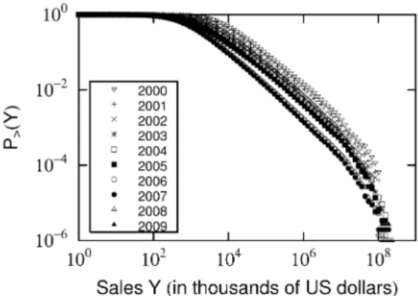
Fig. 2. Distributions of sales Y from 2000 to 2009 in Japan. The average number of firms in the database in each year is 399, 982.
3 Example of Space-Reversal
Quasi-Symmetry
In this section, the mathematical discussion in the pre- vious section is verified by using equal-time data (K, Y ). Here, K and Y are plant assets (P/A) and sales (in thou- sands of US dollars) of firms in the same year, respectively. The authors used the exhaustive global-scale business- finance database ORBIS [40] owned by Hitotsubashi Uni- versity.
First of all, CDFs P>(K) and P>(Y ) follow power laws above size thresholds K0, Y0:
P>(K)∝ K−μK for K > K0, (18) P>(Y )∝ Y−μY for Y > Y0 , (19) respectively. In Figs. 1 and 2, for example, power-law dis- tributions of K and Y in large-scale ranges in Japan were observed, respectively. At the same time, in the joint PDF PJ(K, Y ), symmetry under the exchange of variables Y ↔
4 Atushi Ishikawa et al.: Emergence of power laws with different power-law exponents
Fig. 3.A scatter plot between plant assets (P/A) K and sales Y of firms in 2008 in Japan. The range of K is restricted to the power-law range.
aKYKθK Y was observed as follows: PJ(K, Y ) = PJ(
µ Y aKY
¶1/θKY
, aKYKθK Y) . (20) The authors call this “space-reversal quasi-symmetry.” For example, Fig. 3 shows a scatter plot of (K, Y ) data for firms in 2008 in Japan and the symmetric line log Y = θKY log K + log aKY. The symmetric line was settled by the following steps:
1) The range of a power-law distribution of K was iden- tified by improving the method suggested by Malevergne et al. [41]. Due to the finite-size effect, in a distribution of large-size data, there were firms which deviated from the power law in the right-hand side of the distribution (Figs. 1 and 2). Therefore, an erroneous decision occa- sionally occurred on a size threshold value of a power-law range K0. This did not become a subject of discussion in the analysis of the small-size data used in Ref. [41]. To avoid this kind of erroneous decision, the authors sup- pressed the finite-size effect by thinning observed values. After that, the power-law range was identified by apply- ing the method suggested by Malevergne et al. Detailed discussions were presented in Ref. [42].
2) The power-law range of K was divided into loga- rithmically equal size bins, and the geometric average in each bin was calculated. The symmetric line was decided by applying the least-square method to the geometric av- erages. This method was used in Ref. [16], [28].
There were a predominant number of small-size data points on the left-hand side of the power-law range. In comparison, the number of large-size data points on the right-hand side was small (Fig. 3). To give the same weight to estimations of small- and large-size data points, the au- thors did not apply the least-square method to individual points, but applied geometric averages in logarithmically equal size bins. Using the Kolmogorov-Smirnov (KS) test, we were able to confirm space-reversal quasi-symmetry (20) with respect to the symmetric line decided by this procedure.
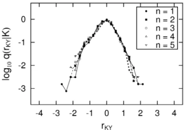
Fig. 4. Conditional PDFs q(rKY|K) of the logarithmic rate rKY = log RKY = log Y /(aKYKθKY). The range of the ini- tial value K is divided into logarithmically equal bins as K∈£104+0.2(n−1), 104+0.2n¢(n = 1, 2, · · · , 5).
Furthermore, let us consider the exchange ratio of vari- ables RKY = Y /(aKYKθKY). It was observed that, above some size threshold K0, the conditional PDF Q(RKY|K) did not depend on the initial value K, as follows:
Q(RKY|K) = Q(RKY) for K > K0 . (21) This is Gibrat’s law in the space direction. For example, Fig. 4 depicts the conditional PDFs Q(RKY|K), which do not depend on the initial value K, in 2008 in Japan .
As just described, power laws, space-reversal quasi- symmetry, and Gibrat’s law were observed in equal-time data (K, Y ). To verify the consistency of the discussion in the previous section, let us confirm Eq. (17), which relates the power-law exponents μ of two power-law distributions to the parameter of space-reversal quasi-symmetry θ. For this section, Eq. (17) is rewritten as
μK = θKYμY . (22)
Empirical data confirmed this relation. For instance, Fig. 5 shows the verification of Eq. (22), using data of firms for twelve countries of the world in 2006. The power-law range of Y was also determined by method 1) [42]. As a result, empirical equal-time data validated the mathematical dis- cussion in the previous section.
4 An Extension of Reversal Quasi-Symmetry
in 3-Dimensions
In the previous section, taking equal-time variables (K, Y ), we observed space-reversal quasi-symmetry (20). This was invariance of the joint PDF with respect to the line log Y = θKY log K + log aKY in the (log K, log Y ) plane. It was shown that space-reversal quasi-symmetry and Gibrat’s law led to power laws of K and Y . Similar analyses were applicable for variables (Y, L) and (K, L), where L was the
Fig. 5.The relation between μK/μY and θK Y for twelve coun- tries in 2006. JP means Japan (723, 109), FR France (887, 142), ES Spain (718, 729), IT Italy (611, 988), RU Russian Federa- tion (548, 086), GB United Kingdom (342, 370), PT Portuguese (280, 941), KR Korea (134, 450), CN China (247, 318), UA Ukraine (252, 144), NO Norway (162, 983) and DE Germany (213, 017). The number in parentheses is the number of firms in the database. Only countries with a sufficient quantity of data were chosen.
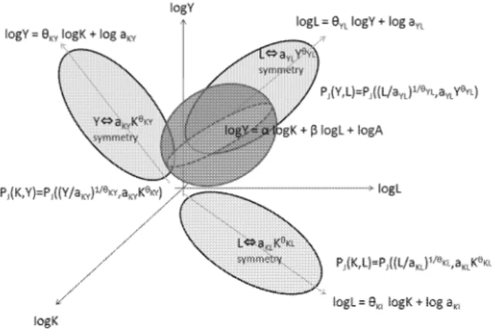
Fig. 6. Three kinds of space-reversal quasi-symmetry in (log K, log Y ), (log Y, log L) and (log K, log L) planes were recognized as maps from symmetry in 3-dimensional space (log K, log L, log Y ).
number of employees. As a result, three kinds of symme- try were confirmed in the (log K, log Y ), (log Y, log L) and (log K, log L) planes. These were considered to be maps from symmetry with respect to a plane in 3-dimensional space (log K, log L, log Y ) (Fig. 6). From this point of view, in this section, we discuss reversal quasi-symmetry of three variables (u1, u2, v).
Let us suppose 3-dimensional reversal quasi-symmetry in the joint PDF PJ(u1, u2, v) as follows:
PJ(u1, u2, v) = PJ(
µ v
Au2θ2
¶1/θ1
,
µ v
Au1θ1
¶1/θ2
, Au1θ1u2θ2) . (23)
This is invariance with respect to a plane:
log v = θ1log u1+ θ2log u2+ log A (24) in 3-dimensional space (log u1, log u2, log v). By rewriting Au2θ2 = a1and paying attention to the first and the third arguments, we can regard Eq. (23), as 2-dimensional re- versal quasi-symmetry (4) in the (log u1, log v) plane:
PJ(u1, v) = PJ( µv
a1
¶1/θ1
, a1u1θ1) . (25) Similarly, by rewriting Au1θ1 = a2 and paying attention to the second and the third arguments, we can regard Eq. (23) as 2-dimensional reversal quasi-symmetry in the (log u2, log v) plane:
PJ(u2, v) = PJ( µv
a2
¶1/θ2
, a2u2θ2) . (26) The disregarding of the second or the first argument cor- responds to the identification with different data points in the second or the first direction, respectively. These are maps from symmetry in the 3-dimensional space to sym- metry in the (log u1, log v) or (log u2, log v) plane.
Reversal quasi-symmetry (25), (26) is invariance un- der exchanges of variables v ↔ a1u1θ1, v ↔ a2u2θ2, re- spectively. If Gibrat’s law is valid, conditional PDFs of the exchange rates of variables R1 = v/(a1u1θ1), R2 = v/(a2u2θ2) obey the following relations:
Q(R1|u1) = Q(R1) , (27) Q(R2|u2) = Q(R2) . (28) With reversal quasi-symmetry of two variables (u1, v) (25) and (u2, v) (26) reduced from symmetry of three variables (u1, u2, v) (23), Gibrat’s laws (27) and (28) led to power- law distributions of (u1, v) and (u2, v). In the empirical data, observations of Eqs. (25)—(28) and the power-law distributions validated the consistency of this discussion. At the same time, using the slopes of symmetric lines θ1, θ2estimated in the joint PDFs PJ(u1, v) and PJ(u2, v) re- spectively, the symmetric plane (24) was able to be identi- fied in 3-dimensional space. The decomposition of reversal quasi-symmetry of three variables to two kinds of symme- try of two variables was useful for this identification.
In the use of empirical data (K, L, Y ), the main point was as follows. There were correlations not only between (K, Y ), but also between (L, Y ) and (K, L), as mentioned in the beginning of this section. If (u1, u2, v) had been taken as (K, L, Y ) directly, the estimated values θ1, θ2
would have been unstable due to multicollinearity. To avoid this problem, the authors introduced variables (Z1, Z2), which did not correlate with each other, by orthogonal transformations of linearly correlated variables as follows:
log Z1= log L σlog L
+ log K σlog K
, (29)
log Z2= log L σlog L −
log K σlog K
. (30)
6 Atushi Ishikawa et al.: Emergence of power laws with different power-law exponents
Fig. 7. A scatter plot between Z1 and Y of firms in 2008 in Japan.
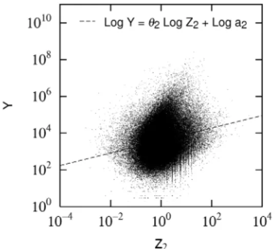
Fig. 8. A scatter plot between Z2 and Y of firms in 2008 in Japan.
Here, σlog K and σlog L are standard deviations of log K and log L, respectively.
Let us verify the analytical discussion with empirical data (Z1, Z2, Y ). In this case, Eqs. (25) and (26) showed space-reversal quasi-symmetry with respect to the follow- ing lines:
log Y = θ1log Z1+ log a1, (31) log Y = θ2log Z2+ log a2 (32) in the (log Z1, log Y ) and (log Z2, log Y ) planes, respec- tively. For instance, Figs. 7 and 8 depict scatter plots (Z1, Y ), (Z2, Y ) of data for firms in Japan in 2008. Space- reversal quasi-symmetry with respect to lines (31) and (32) was confirmed by the KS test. The symmetric lines were determined in the same manner as in the previous section. Figs. 9 and 10 show the verification of Gibrat’s laws observed in the distributions of the change rates of the variables. Power-law distributions of Z1, Z2 and Y were also observed.
Fig. 9. Conditional PDFs q(r1|Z1) of the logarithmic rate r1 = log R1 = log Y /(a1Z1θ1). The range of the initial value Z1 is divided into logarithmically equal bins as Z1 ∈
£100.5(n−1), 100.5n¢(n = 1, 2, · · · , 5).
Fig. 10. Conditional PDFs q(r2|Z2) of the logarithmic rate r2 = log R2 = log Y /(a2Z2θ2). The range of the initial value Z2 is divided into logarithmically equal bins as Z2 ∈
£10−2+0.4(n−1), 10−2+0.4n¢(n = 1, 2, · · · , 5).
The plane (24) in 3-dimensional space was expressed as
log Y = α log K + β log L + log A (33) by transformations of variables (29) and (30). The param- eters were given by
α = θ1− θ2 σlog K
, β = θ1+ θ2 σlog L
. (34)
Under these parameterizations, joint PDF PJ(K, L, Y ) in- variance under the exchange of variables with respect to the plane (33) in 3-dimensional space was justified. This symmetric plane was recognized as the Cobb-Douglas pro- duction function:
Y = AKαLβ , (35)
which is an optimized function with empirical data in eco- nomics [43], [44].
5 Conclusion
In this study, to explore the emergence of power laws in social and economic phenomena, we discussed the mecha- nism by which reversal quasi-symmetry and Gibrat’s law lead to power laws with different power-law exponents. The power-law exponents were related to each other by the parameter of reversal quasi-symmetry. Reversal quasi- symmetry was invariance under the exchange of variables in the joint PDF. Gibrat’s law meant that the conditional PDF of the exchange rate of variables did not depend on the initial value. By using empirical worldwide data for firm size, related to categories such as plant assets K, the number of employees L, and sales Y in the same year, re- versal quasi-symmetry, Gibrat’s laws, and power-law dis- tributions were observed. Most importantly, we confirmed relations between power-law exponents in the same year. This result could probably not have been verified without a database of different countries for the firms, since the annual change of power-law exponents in a single country was quite small [18].
The authors have discussed the existence of reversal quasi-symmetry of three variables. We showed that re- versal quasi-symmetry of three variables could be decom- posed to two kinds of reversal quasi-symmetry of two vari- ables. By using empirical data (K, L, Y ), two kinds of de- composed reversal quasi-symmetry of two variables were observed. At the same time, Gibrat’s laws and power-law distributions were also confirmed. These observations jus- tify the existence of reversal quasi-symmetry of three vari- ables. Note that, in the analysis, the variables (K, L) were changed to (Z1, Z2) to eliminate the correlation between K and L that caused multicollinearity. The authors claim that the plane in 3-dimensional space (log K, log L, log Y ), with respect to which the joint PDF PJ(K, L, Y ) is invari- ant under the exchange of variables, fit the empirical data, at least in the large-scale ranges where power laws were observed. This is known as the Cobb-Douglas production function Y = AKαLβ, which is frequently hypothesized in economics.
Some interesting issues remain. In analyses of firm size data for countries worldwide, the magnitude relation among power-law exponents was found to be μL > μY > μK. At the same time, the magnitude relation between parameters in the Cobb-Douglas production function was also found to be β > α. With respect to the output elas- ticities of capital α and labor β, constant returns to scale α + β = 1 were approximately observed [45]. These rela- tions can be explained by space-reversal quasi-symmetry. Furthermore, if α and β are fixed in some category such as country, industry sector and so forth, the total factor productivity A of each firm can be calculated by using the Cobb-Douglas production function Y = AKαLβ. The total factor productivity A is considered to be the technol- ogy of the firm which contributes to Y , except for assets K and labor L. The distribution of A in some categories such as country, industry sector, and so on should be studied further [45]. These issues will be discussed in a forthcom- ing paper [46].
Acknowledgment
This work was supported in part by a Grant-in-Aid for Scientific Research (C) (No. 20510147) and Creative Sci- entific Research (No.18GS0101) from the Ministry of Ed- ucation, Culture, Sports, Science and Technology, Japan.
References
1. H. E. Stanley, Introduction to Phase Transitions and Criti- cal Phenomena(Claredon Press, Oxford, 1971).
2. V. Pareto, Cours d’Economique Politique (Macmillan, Lon- don, 1897).
3. M. E. J. Newman, Contemporary Physics 46 (2005) 323. A. Clauset, C. R. Shalizi and M. E. J. Newman, SIAM Re- view 51 (2009) 661.
4. E. Bonabeau and L. Dagorn, Phys. Rev. E 51 (1995) R5220. 5. S. Render, Eur. Phys. J. B4 (1998) 131.
6. M. Takayasu, H. Takayasu and T. Sato, Physica A 233 (1996) 824.
7. A. Saichev, Y. Malevergne and D. Sornette, Theory of Zipf ’s law and beyond, Lecture Notes in Economics and Mathemat- ical Systems, p. 632 (Springer, 2009).
8. T. Kaizoji, Physica A 326 (2003) 256. 9. T. Yamano, Eur. Phys. J. B 38 (2004), 665. 10. A. Ishikawa, Physica A 371 (2006) 525;
A. Ishikawa, Prog. Theor. Phys. Supple. No. 179 (2009) 103. 11. R. N. Mantegna and H. E. Stanley, Nature 376 (1995) 46. 12. R. L. Axtell, Science 293 (2001) 1818.
13. B. Podobnik, D. Horvatic, A. M. Petersen, B. Uro˘sevi´c and H. E. Stanley, Proc. Natl. Acad. Sci. USA 107 (2010) 18325. 14. D. Fu, F. Pammolli, S. V. Buldyrev, M. Riccaboni, K. Ma- tia, K. Yamasaki and H. E. Stanley, Proc. Natl. Acad. Sci. 102 (2005) 18801.
15. B. Podobnik, D. Horvatic, F. Pammolli, F. Wang, H. E. Stanley and I. Grosse, Phys. Rev. E 77 (2008) 056102. 16. K. Okuyama, M. Takayasu and H. Takayasu, Physica A
269 (1999) 125.
17. J. J. Ramsden and Gy. Kiss-Hayp´al, Physica A 277 (2000) 220.
18. T. Mizuno, M. Katori, H. Takayasu and M. Takayasu, Em- pirical Science of Financial Fluctuations - The Advent of Econophysics(Springer Verlag, Tokyo, 2002) 321.
19. E. Gaffeo, M. Gallegati and A. Palestrinib, Physica A 324 (2003) 117.
20. J. Zhang, Q. Chen, and Y. Wang, Physica A 388 (2009) 2020.
21. H. Kesten, Acta Math. 131 (1973) 207.
22. M. Levy and S. Solomon, Int. J. Mod. Phys. C7 (1996) 595.
23. D. Sornette and R. Cont, J. Phys. I7 (1997) 431.
24. H. Takayasu, A. Sato and M. Takayasu, Phys. Rev. Lett. B79 (1997) 966.
25. Y. Fujiwara, W. Souma, H. Aoyama, T. Kaizoji and M. Aoki, Physica A321 (2003), 59.
Y. Fujiwara, C.D. Guilmi, H. Aoyama, M. Gallegati and W. Souma, Physica A335 (2004), 197.
26. R. Gibrat, Les inegalites economiques (Sirey, Paris, 1932). 27. J. Sutton, J. Econo. Lit. 35 (1997) 40.
28. H. Watanabe, H. Takayasu and M. Takayasu, Statisti- cal Studies on Interrelationships of Financial Indicators of Japanese Firms, The Physical Society of Japan 2009 Autumn Meeting, in Japanese.
8 Atushi Ishikawa et al.: Emergence of power laws with different power-law exponents
29. C. K¨uhnert, D. Helbing and G. B. West, Physica A363 (2006) 96.
30. X. Gabaix, Annu. Rev. Econ. 1 (2009) 255.
31. A. H. Jessen and T. Mikosch, Inst. Math. 94 (2006) 171. 32. C. W. Cobb and P. H. Douglas, American Economics Re-
view, 18 (1928) 139.
33. E. J. Bartelsman and P. J. Dhrmes, Journal of Productiv- ity Analysis 9(1) (1998) 5.
34. B. Y. Aw, X. Chen and M. J. Roberts, Journal of Devel- opment Economics 66(1) (2001) 51.
35. H. S. Houthakker, Review of Economics Studies vol. 23, no. 1 (1955) 27.
36. S. Rosen, Economica, vol. 45, no. 179 (1978) 235. 37. C. I. Jones, Quarterly Journal of Economics, vol. 120, no.
2 (2005) 517.
38. J. Growiec, Economics Letters 101 (2008) 87.
39. J. Growiec, A New Class of Production Functions and an Argument Against Purely Labor-Augmenting Technical Change, to appear in International Journal of Economic The- ory.
40. Bureau van Dijk, http://www.bvdinfo.com/Home.aspx. 41. Y. Malevergne, V. Pisarenko and D. Sornette, Phys. Rev.
E 83 (2011) 036111.
42. S. Fujimoto, A. Ishikawa, T. Mizuno and T. Watanabe, A New Method for Measuring of Firm Size Distributions, Economics -Special Issues New Approaches in Quantitative Modeling of Financial Markets- Discussion Paper (2011) 2011 - 29.
43. W. Souma, Y. Ikeda, H. Iyetomi and Y. Fujiwara, Eco- nomics -Special Issues Reconstructing Macroeconomics- vol. 3 (2009) 2009 - 14.
44. Y. Ikeda and W. Souma, Prog. Theor. Phys. Supple. No. 179 (2009) 97.
45. T. Watanabe, T. Mizuno, A. Ishikawa and S. Fujimoto, A New Method for Specifying Functional Forms of Produc- tion Functions, to appear in The Economic Review (Keizai Kenkyuu, in Japanese).
46. T. Mizuno, T. Watanabe, A. Ishikawa and S. Fujimoto, in preparation.