つくばリポジトリ MNRAS 461 1 967

(1)

page r ange

967- 983

year

2016- 09

権利

Thi s ar t i c l e has been ac c ept ed f or publ i c at i on

i n M

ont hl y N

ot i c es of t he Royal As t r onom

i c al

Soc i et y

( C) 2016 The Aut hor s . Publ i s hed by O

xf or d

U

ni ver s i t y Pr es s on behal f of t he Royal

As t r onom

i c al Soc i et y. Al l r i ght s r es er ved.

U

RL

ht t p: / / hdl . handl e. net / 2241/ 00144241

(2)

Advance Access publication 2016 June 8

Relativistic jet feedback in high-redshift galaxies – I. Dynamics

Dipanjan Mukherjee,

1‹

_{Geoffrey V. Bicknell,}

1

_{Ralph Sutherland}

1

_{and Alex Wagner}

2

1_{Research School of Astronomy and Astrophysics, Australian National University, Canberra, ACT 2611, Australia} 2_{Center for Computational Sciences, University of Tsukuba, 1-1-1 Tennodai, Tsukuba, Ibaraki 305-8577, Japan}

Accepted 2016 June 3. Received 2016 June 3; in original form 2016 April 14

A B S T R A C T

We present the results of 3D relativistic hydrodynamic simulations of interaction of active galactic nucleus jets with a dense turbulent two-phase interstellar medium, which would be typical of high-redshift galaxies. We describe the effect of the jet on the evolution of the density of the turbulent interstellar medium (ISM). The jet-driven energy bubble affects the gas to distances up to several kiloparsecs from the injection region. The shocks resulting from such interactions create a multiphase ISM and radial outflows. One of the striking result of this work is that low-power jets (Pjet1043ergs−1), although less efficient in accelerating clouds, are trapped in the ISM for a longer time and hence affect the ISM over a larger volume. Jets of higher power drill through with relative ease. Although the relativistic jets launch strong outflows, there is little net mass ejection to very large distances, supporting a galactic fountain scenario for local feedback.

Key words: hydrodynamics – methods: numerical – galaxies: evolution – galaxies:

high-redshift – galaxies: ISM – galaxies: jets.

1 I N T R O D U C T I O N

Feedback from active galactic nuclei (AGNs) has long been identi-fied as playing an important role in the evolution of galaxies (e.g. Silk & Rees1998; Di Matteo, Springel & Hernquist2005; Bower et al.2006; Croton et al.2006; Schawinski et al.2007). It has been proposed that momentum-driven or energy-driven jets and winds powered by the central black hole significantly affect the gas con-tent and star formation of galaxies (e.g. Silk & Rees1998; Di Matteo et al.2005; Murray, Quataert & Thompson2005; Ciotti, Ostriker & Proga2010; Dubois et al.2013). However, only a few papers have addressed the complex nature of the interaction of such winds with a dense multiphase interstellar medium (ISM; see for example Hopkins & Elvis2010; Gabor & Bournaud2014; Hop-kins et al.2016). Oppenheimer et al. (2010) and Dav´e, Finlator & Oppenheimer (2012) have considered a galactic fountain scenario in which there is a recurrent cycle of blow out of gas and its subsequent infall. However, for galaxies of masses1011_M

⊙, Oppenheimer

et al. (2010) find the need for an additional quenching mechanism, possibly due to AGN, to suppress excess accretion of gas and star formation in order to match the galaxy stellar mass function.

Our work concentrates on the role of radio galaxies in AGN feed-back, specifically the role played by their relativistic jets. This is motivated by investigations of the radio/optical luminosity function, which have shown that the probability of a galaxy being a radio source increases with optical luminosity (Auriemma et al.1977; Sadler, Jenkins & Kotanyi1989; Ledlow & Owen1996; Best et al.

⋆_E-mail:_{[email protected]}

2005; Mauch & Sadler2007). It is the most luminous part of the op-tical luminosity function where discrepancies between hierarchical models of galaxy formation and observation are most apparent (e.g. Croton et al.2006) and considerations of the radio–optical luminos-ity function indicate that it is in the optically luminous galaxies in which radio sources are most likely to play an important role. This reinforces the potential role of relativistic jets in AGN feedback. Nevertheless, not every optically luminous galaxy is a radio galaxy, indicating that radio galaxies are an intermittent phenomenon and that jet feedback is also necessarily intermittent.

Effects of feedback from relativistic jets have been investigated more in the context of heating the intracluster medium to prevent catastrophic cooling and accretion of gas to the cluster centre (e.g. Binney & Tabor1995; Soker et al.2001; Gaspari, Ruszkowski & Sharma2012). However, relativistic jets are also expected to be one of the major drivers of feedback on galactic scale, as supported by several observational evidences of jet-ISM interaction (a few recent works being Nesvadba et al. 2007, 2008, 2011; Morganti et al.

2013,2015; Dasyra et al.2014,2015; Ogle, Lanz & Appleton2014; Tadhunter et al.2014; Lanz et al.2015b; Collet et al.2016; Mahony et al.2016). However, only a few theoretical papers (Sutherland & Bicknell 2007; Gaibler, Khochfar & Krause2011; Wagner & Bicknell2011b; Gaibler et al.2012; Wagner, Bicknell & Umemura

2012) have addressed the question of how a relativistic jet interacts with a multiphase ISM of the host galaxy, and over what scales such interactions are relevant.

In this work, we extend the results presented in Wagner & Bicknell (2011a, hereafterWB11) and Wagner et al. (2012, here-afterWBU12). The simulations presented in those papers consist of gas distributed on a scale_∼1 kpc in the form of a two phase

at University of Tsukuba on October 30, 2016

http://mnras.oxfordjournals.org/

(3)

were also established.

In WB11 and WBU12, gas was considered to be ‘dispersed’ when its radial velocity exceeds the velocity dispersion of the host galaxy. However, while useful, this approach does not fully address the ultimate fate of potentially star-forming gas interacting with relativistic jets. Is it completely ejected from the atmosphere of the host – or does it simply become turbulent – impeding for a time, but not indefinitely, the formation of new stars? What happens when the jet breaks free of the dense gas surrounding the nucleus? Also, in WB11andWBU12, the dense clouds were static without any associated velocity dispersion.

Hence, in this paper, we present the next step in this program of simulations, adding the following significant features. (1) A grav-itational field typical of that of an elliptical galaxy consisting of luminous and dark matter (see Sutherland & Bicknell2007). (2) An internal velocity dispersion for the dense thermal gas; this is used to establish an initial turbulent ISM consistent with observations of high-redshift elliptical galaxies (F¨orster Schreiber et al.2009; Wisnioski et al.2015). (3) Both phases of the ISM, consisting of hot gas at around the virial temperature and the warm gas at a temperature of about 104_{K are distributed consistently with the}

gravitational field. This restricts the dense, warm gas to a region of order the core radius of the stellar distribution, thereby defining the region for jet break and the time-scale over which the jet signifi-cantly affects the distribution and kinematics of the dense gas. (4) A scale of 5 kpc for the simulations, significantly larger than the 1 kpc scale in our previous work.

In the following section (Section 2), we describe the simulation setup in detail and in Section 3 we document how the ISM is settled from its initial configuration. In Section 4, we examine the impact of a relativistic jet with power 1045_ergs−1_{on the turbulent ISM. We}

describe the evolution of the ISM density and the multiphase nature of the ISM resulting from shocks driven by the jet. In Section 5, we examine the dependence of morphology on jet power by comparing the results of four jet simulations with jet kinetic powers ranging from 1043 _{to 10}45_{erg s}−1_{. We emphasize the efficiency of}

low-power jets in coupling with the ISM. In Section 6, we consider the energetics of the disturbed ISM, including a discussion of the galactic fountains revealed by our simulations and summarize the results in Section 7.

2 S I M U L AT I O N S E T U P

2.1 Gravitational potential

We model the gravity of the host galaxy by prescribing a spherically symmetric isothermal potential as a function of radiusrfor both the dark matter and baryonic components. Let the velocity dispersions of the dark and baryonic matter be σDandσB, respectively, the

2.2 Initialization of the simulation

We initialize the simulation domain with a two phase, spheri-cally distributed medium following the approach of Sutherland & Bicknell (2007),WB11andWBU12. The density consists of an isothermal hot (T_∼107K; typical of galaxy clusters and elliptical galaxies, Allen et al.2006; Croston et al.2008; Diehl & Statler

2008; Maughan et al.2012; Goulding et al.2016) halo in hydro-static equilibrium and a dense warm (T3.4_×104_{K) turbulent and}

inhomogeneous gas. The density of the hot halo (HH) is described by

nh=n0exp

−μm_k aφ BT

, (2)

wheren0is the central number density,μ= 0.6165 is the mean

molecular weight andmais the atomic mass unit. For this work,

we choosen0=0.5 cm−3, similar to values of central gas densities

inferred from X-ray observations of diffuse haloes around elliptical galaxies and galaxy clusters (Allen et al.2006; Croston et al.2008; Goulding et al.2016). The pressure,p₌nhkBT, is evaluated from

the specified temperature and equation (2).

The density in the warm phase is distributed as a fractal with a single point lognormal density distribution and a Kolmogorov power spectrum

D(k)₌

4π_k2_F(k)F∗(k)dk_∝k−5/3, (3)

F(k_{) being the Fourier transform. The fractal density distribution is}

created using the publicly availablePYFC1routine (written by Alex

Wagner) with meanμPDF₌1 andσPDF2 =5. The resultant

distri-bution (nfractal) is then apodized to represent a spherical isotropic,

turbulent distribution in the gravitational potential, as follows. Let σtbe the turbulent velocity dispersion of the warm gas andTwits

temperature, withσ_t2_≫3kB/μm. Then the density distribution of

warm gas is given by

nw(r, z)=nfractal×nw0exp

−φ(r, z)−φ(0,0)

σt2

, (4)

where nw0 is the number density at (0, 0) (see Sutherland &

Bicknell2007, for details). For our simulations, we assume the mean central density of the warm clouds to be _∼100–300cm−3_,

which is consistent with typical densities of ISM inferred in high-Z galaxies (see e.g. Shirazi, Brinchmann & Rahmati2014; Sanders et al.2016). Tables1and2present the values of the parameters used in our simulations. The warm phase is initialized to be at the same pressure as the HH at a given location, so that the entire domain is in pressure equilibrium. A lower bound is placed on the density of the

1_{https://pypi.python.org/pypi/pyFC}

(4)

Table 1. Parameters of the ambient gas and gravitational poten-tial common to all simulations.

Parameters Value

Baryonic core radius rB 1 kpc

Baryonic velocity dispersion σB 250 km s−1

Ratio of DM to Baryonic λ 2

core radius

Ratio of DM to Baryonic κ 10

velocity dispersion

Halo Temperature Th 107K

Halo density at r₌0 n0 0.5 cm−3

Turbulent velocity dispersiona _σ

t 250 km s−1

of warm clouds

Note. a_{Defines the extent of the cloud distribution in} equation (4).

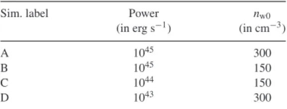
Table 2. Jet simulations.

Sim. label Power nw0

(in erg s−1₎ _{(in cm}−3₎

A 1045 ₃₀₀

B 1045 ₁₅₀

C 1044 ₁₅₀

D 1043 ₃₀₀

warm phase corresponding to a temperature ofTcrit=3.4×104K,

beyond which the clouds are considered to be thermally unstable; gas in those cells is replaced by hot gas.

2.3 Jet parameters

Following Bicknell (1995), we express the kinetic jet power as fol-lows. The jet parameters are the pressurepjet, velocity with respect

to the speed of lightβ ₌ v/c, Lorentz factorŴ₌1/ 1₋β2, cross-sectional areaAjet, adiabatic indexγadand the density

param-eterχ, which is the ratio of the rest mass energy to the enthalpy. The jet power is

Pjet=

γad

γad−1cpjetŴ 2

βAjet

1₊Ŵ−1 Ŵ χ

. (5)

The parameterχis given by

χ₌

γad−1

γad

ρc2 pjet

. (6)

In our simulations, we inject the jet at the lowerzboundary of the computation domain,z₌z0, assuming conical expansion between

z₌0, the location of the black hole andz₌z0. The radius of the

inlet region is constrained by the grid resolution such that at least 10 cells cover the jet inlet. For our simulations, we set the inlet radius to be 30 pc. The jet is injected with a half opening angle of 10◦_so

thatz0=. 170 pc. We initialize the jet with a given kinetic power

(Pjet) and Lorentz factor (Ŵ). We assume the jet to be in pressure

equilibrium with the gas at the inlet, thus constraining the parameter χ from equation (5); this in turn defines the jet density. For the simulations presented here,χ5. We assume an ideal equation of state withγad=5/3, which is a reasonable approximation for a

relativistic gas in withχ_≫1 (Synge1957; Mignone & McKinney

2007). Also, a non-relativistic ideal equation of state is a better descriptor of the thermal gas inside the simulation domain and it is mainly the effect on the thermal gas in which we are interested.

Adoption of such a value ofχraises questions about jet composi-tion, which is not very well constrained for extragalactic jets (see the discussion in Worrall2009). An electron–positron jet would haveχ

∼1 and this value would be obtained if the jet were overpressured

with respect to the ISM by a factor of 5. On the other hand, if the jet is in pressure equilibrium with the ISM, then it may entrain some thermal material as it travels to_∼170 pc from the nucleus, which is the starting point of our simulation.

As Worrall (2009) has noted, the dominant contribution in ra-dio power, comes from sources around the FRI/FRII break, cor-responding to the peak of the curveP(P), wherePis the radio power and(P) is the number density of sources per unit logP. The relationship between radio power and jet power is not straightfor-ward (see e.g. Godfrey & Shabala2016). Nevertheless, Rawlings & Saunders (1991) identified 1043_{erg s}−1_{as the low end of the FRII}

population; Bicknell (1995) found the FRI/FRII break jet power to be_∼2_×1042_{erg s}−1_{. Hence, in this paper, we concentrate on jet}

powers ranging from 1043_{to 10}45_{erg s}−1_{, whilst noting that}

inves-tigations of jets of both lower and higher powers are certainly of interest.

2.4 PLUTOsetup

We perform 3D relativistic hydrodynamic simulations using the

PLUTOcode’s Relativistic Hydrodynamic (RHD) module (Mignone

et al.2007). We use a Cartesian geometry with a uniform grid of resolution 6 pc for the central 3 kpc, followed by a geometrically stretched grid with stretching ratio of_∼1.0128, extending up to

±2.4 kpc along thex–ydirections and_∼5.2 kpc in thezdirection. The total number of grid points along thex–y–zdirections are 668

×668×640. We use the piecewise parabolic method (Colella &

Woodward1984; Mart´ı & M¨uller1996) for the reconstruction step of the Godunov scheme, which is well suited for non-uniform grids. The time evolution is carried out using third-order dimensionally unsplit Runge–Kutta method. The HLLC Riemann solver (Toro

2008) is used for solving the hydrodynamic equations.

The non-equilibrium cooling function was evaluated from the Mappings 5.1 code (Sutherland et al., in preparation). This code is the latest version of theMAPPINGS4.0 code described in Nicholls

et al. (2013) and Dopita et al. (2013), and includes numerous up-grades to both the input atomic physics (CHIANTI v8, Del Zanna et al.2015) and new methods of solution. MAPPINGS V includes

up to 30 elements from H to Zn, of which about 10–15 provide most of the cooling. For most temperatures, oxygen and iron dom-inate the cooling except in some temperature regimes (very hot and 104 _{K), where collisional cooling of hydrogen and helium}

are key. In these models, we have adopted solar abundances from Asplund et al. (2009) as representative of metallicities of larger host galaxies.

The cooling function is constructed by having the plasma initially fully ionized at an extremely high temperature, 109_{K, where the}

thermal cooling is primarily free–free emission, and the ions are fully stripped. This high temperature is outside the range expected in the simulations, and in a regime where cooling is unimportant. Without more detailed microphysics, such as a fully relativistic treatment of free–free emission for example, theMAPPINGScooling

functions above_∼108.5_{K or so are not intended for detailed model}

fitting, but serve as a smooth upper boundary to the cooling which improves the numerical properties of the cooling treatment. For gas belowT<104K cooling was deactivated.

The plasma in theMAPPINGSmodel is allowed to cool in a

time-dependent isobaric way, similar to a post-shock flow (Sutherland &

(5)

Figure 1. Density (log [n(cm−3_{)]) in the}_x_–_z_{plane for settling turbulent ISM at two different times. The ISM develops a filamentary structure, typical of a} turbulent medium.

Dopita1993; Allen et al.2008). Cooling down to 106_{K proceeds}

with equilibrium ionization and cooling, until the cooling becomes rapid compared to the recombination time-scales and the ionization lags behind, being more ionized at a given temperature than in equilibrium. Below 106_{K, the cooling rates increase to a maximum}

around_∼105_{K, before falling rapidly below 10}4_{K. At each point,}

the full ionization state including electron densities and atomic level populations, are solved, allowing the cooling and a simple equation of state to be inferred from the self-consistently changing mean molecular weightμ(T). The gas is assumed to be atomic, and to have an ideal adiabatic index of 5/3. The temperature-dependent cooling function and mean molecular weight thus obtained were tabulated as a function of the ratio of pressure and density (p/ρ), which are

PLUTOprimitive variables. The cooling losses ([ρ/μ(T)]2(T)) for each cell in thePLUTO domain were applied by interpolating the

cooling function and mean molecular weight from the tabulated list.

3 S E T T L I N G O F I S M

(i) Filamentary ISM: we initialize the velocity in the warm cloudy medium with a turbulent velocity distribution, modelled as a ran-dom Gaussian variate for the three velocity components with a Kolmogorov spectrum in Fourier space. We set the velocity disper-sion of the clouds higher than that of the baryonic disperdisper-sion of the galaxy and let the clouds settle in the potential. The fractal clouds disperse and shear due to the turbulent motions and cloud–cloud collisions. The clouds eventually condense into filaments, typical of a turbulent medium (e.g. Federrath & Banerjee2015; Federrath

2016) as shown in Fig.1. After_∼1 Myr, the turbulent distribution settles into a two phase medium (see Fig. 1) characterized by a distribution of warm filaments extending up to_∼2 kpc and an HH extending to larger radii.

(ii) Density PDF and two phase ISM: in Fig. 2, we show the volume-weighted probability distribution function (PDF)2 _of

the density at different times of the simulation. Initially (t₌0), the

2_{The volume-weighted PDF of variable is constructed by evaluating the}

histogram and counting the fractional volume of a simulation cell as the weights for a histogram bin.

Figure 2. The PDF of the density (log [n(cm−3_{)]) for a settling ISM without}

jet, att=0 (dash–dotted in blue),t=1.65 Myr (dashed in green) andt=

2.66 Myr (solid red). The black dotted lines represent a fit to the high-density end of the PDF following equation (A7).

density PDF shows two distinct distributions: (a) the warm fractal clouds with high density, (b) a low-density HH. As the ISM evolves under the influence of the turbulent velocity field and gravity, the density PDF changes due to shearing of the clouds. The density PDF converges well after 1 Myr into a two component PDF corre-sponding to a two phase medium. The turbulent motions result in stripping of the dense clouds, lowering the mean of the high-density component of the PDF. The dispersed cloud mass forms a denser halo of gas near the central region.

Density structures formed as a result of hierarchical turbulent processes are expected to exhibit a lognormal probability distri-bution (e.g. Vazquez-Semadeni1994; Padoan, Jones & Nordlund

1997; Klessen2000). However, recent simulations have shown sig-nificant deviation from a lognormal behaviour in the tail of the distribution (Federrath et al.2010; Konstandin et al.2012; Feder-rath & Klessen2013; Federrath & Banerjee2015). Hopkins (2013) has shown that a lognormal-like distribution modified by the influ-ence of intermittency from turbulent shocks is a better descriptor of the PDF in such cases (see Appendix A for a brief summary of the analytical expressions). For our simulations, we find the Hopkins

(6)

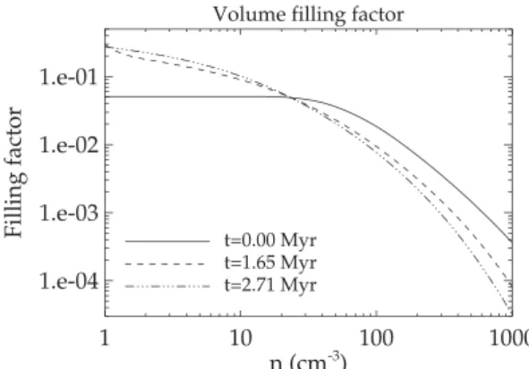
Figure 3. The volume filling factor as a function of density (in cm−3_{) for} a settling ISM.

Figure 4. Comparison of the dispersion of Vx (in kms−1) for different

simulations.σin(in kms−1) is the initial velocity dispersion,nw0(in cm−3)

the mean central density of the warm phase,σB(in kms−1) is the dispersion

of the baryonic component of the gravitational potential andαis the exponent

for a power-law fit to the profiles (σvx∝tα).

function to provide a good fit to the high-density component of the PDFs. For example, the black-dotted line in Fig.2shows the Hopkins function with parameters ¯ρ₌15 cm−3_,_σ

ρ=39.78cm−3, η₌0.08, which provides a good fit to the high-density portion of the PDF att_∼2.7 Myr. For the rest of the paper, we have used the Hopkins function to fit the high-density end of the density PDF and compare the statistics of the ISM under different conditions.

(iii) Volume filling factor: in Fig.3, we show the change in the volume filling factor, defined as the total volume occupied by the gas beyond a threshold density, plotted as a function of density. At t₌0, the volume filling factor forn>10 is0.045. As the clouds shear and settle into filaments, the filling factor is lowered for the high-density cores as the some of the warm gas is dispersed.

(iv) Decay of turbulence: as the clouds settle, the velocity dis-persion decreases as a power law with time. A power-law decay of velocity dispersion (with exponent_∼1.2–2) is typical of hydrody-namic supersonic turbulence (Mac Low et al.1998; Stone, Ostriker & Gammie1998). The rate of decay does not depend on the initial velocity dispersion. For example, as shown in Fig.4, the rate of decay forσin=500 andσin=300 for the samenw=300 is

simi-lar (with the power-law exponentα_{∼ −}0.58. However, as a result of the presence of atomic cooling and external gravity, the rate of settling depends on the mean cloud density and the potential of the galaxy. The settling rate is slower for lower mean cloud density and a gravitational potential with higher stellar dispersion.

Table 3. Coefficients of the fit to the density PDF in Fig.7 following equation (A7).

Zjethead ρ¯ σρ η ρ˜>10

(in kpc) (in cm−3₎a _{(in cm}−3₎b _{(in cm}−3₎c

0 21.38 52.68 0.14 50

1 18.42 44.17 0.14 43.96

3 15.73 27.9 0.12 33.56

5 13.21 20.52 0.17 29.5

Notes.aMean density for the PDF.

b_{Standard deviation of variable}_ρ_{, which is related to the standard deviation}

ins=lnρas in equation (A8).

c_{Volume-weighted mean of density for}_n_>_{10 cm}−3_{. This gives a measure}

of the mean density of the high-density filaments.

4 J E T S I M U L AT I O N S

4.1 Evolution of the density of the ISM

We first let the ISM settle into a turbulent filamentary structure with a velocity dispersion_∼100–150 km s−1_{, which is typical of}

high-redshift galaxies (F¨orster Schreiber et al. 2009; Wisnioski et al.

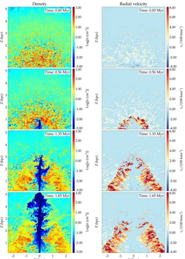
2015). We then inject the relativistic jet whose parameters are de-scribed in Section 2.3. We list the simulations performed with jets interacting with the turbulent ISM in Table 2. In Figs5 and 6, we present the evolution of the density, radial velocity, pressure and temperature of the ISM for simulation A. The jet is initially impeded by the dense filaments (Fig.5) and passes through a flood-channel phase as described in previous works (Sutherland & Bicknell2007;

WB11;WBU12), seeking the paths of least resistance as it drives an energy bubble through the ISM.

The jet shears the dense filaments as it clears its path. The effect of shearing of the dense cores is well demonstrated through the evolution of the density PDF shown in Fig.7. The high-density tail of the PDF is significantly reduced as the jet-driven bubble shears the clouds. There is a subsequent enhancement of the PDF atn_∼ 10–100 cm−3_{, which occurs both as a result of compression of}

low-density gas from the forward shock and also of fragmentation of the dense filaments. Coefficients of fits (following equation A7) to the high-density end of the PDF are listed in Table3. The density PDF converges after the jet breaks out (jet head3 kpc) and decouples from the ISM, proceeding along the cleared path.

The duration of the flood-channel phase of the jet evolution de-pends upon the mean density and filling factor of the ISM, as pre-viously discussed inWBU12. Clouds with denser cores are less ablated and more efficiently impede the progress of the jet. In Fig.8, we present the density for simulation B (Table2), where a jet of power 1045 _ergs−1 _{passes through a medium with lower}

mean density (nw0=150 cm−3) compared to that of simulation A.

We note that the jet breaks out of the warm dense gas much faster, in comparison to simulation A.

4.2 Evolution of the energy bubble

The confined jet creates an expanding energy bubble. A fast moving forward shock first sweeps through the filaments heating the gas to

∼105K (see Fig.6). The forward shock is followed by a slower

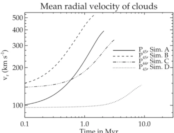
moving region of nearly homogeneous high pressure, defining the energy bubble (see Fig.6). The energy bubble shears the dense fil-aments as it expands into the ISM, accelerating the dense clouds to radial velocities in excess of_∼300 kms−1_{(as shown in Fig.}₉_{), as}

also reported earlier inWBU12. Some of the clouds are dragged

(7)

Figure 5. Left: density (in cm−3_{) in the}_x_–_z_{plane at different times for simulation A (Table}₂_{). Right: radial velocity (in units of 100 kms}−1_{) at the}

same time as left. Dense clouds are pushed radially outwards to several hundred kms−1_{. Low-density ablated cloud mass is accelerated to speeds exceeding}

1000 kms−1_.

(8)

Figure 6. Left: temperature [log (T), withTin Kelvin] in thex–zplane at times same as in Fig.5. Right: pressure [log (p/p0),p0=9.2×10−4_{dynes cm}−2_].

The second panel on the left shows the location of the forward shock (T∼105_{K) preceded by the energy bubble (}_T_>₁₀6_{). Corresponding features can be}

identified in the plot of the pressure on the right. High-pressure knots from recollimation shocks can be clearly identified in the third and fourth panels on the right.

(9)

Figure 7. The evolution of the density PDF as the jet evolves with time

and breaks out of the dense central region after a height ofz∼3 kpc. The

density PDF converges after jet break out as the jet decouples from the ISM.

radially inwards by the backflow near the jet axis. The low-density ablated cloud mass is swept up by the expanding bubble to veloc-ities higher than1000 kms−1_{, flowing out through the channels}

between the denser clouds (see Fig.5).

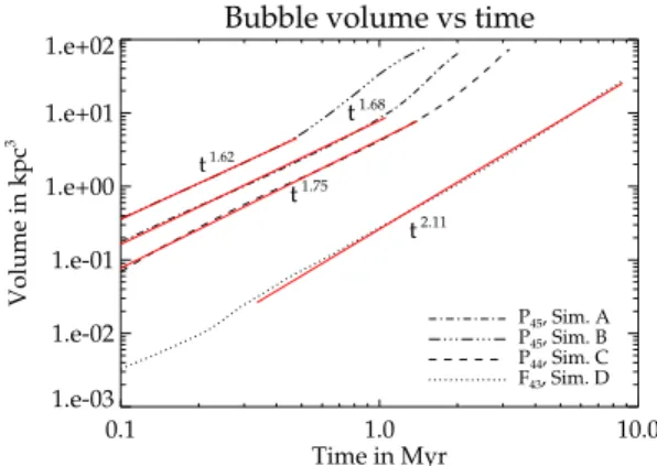
In Figs10and11, we show the evolution of the mean pressure inside the energy bubble and the volume of the bubble. For high-power jets (Pjet 1044 ergs−1), initially the high-pressure bubble

expands nearly adiabatically. The power-law evolution of the pres-sure in Fig.10can be understood by solving the energy equation for an adiabatically expanding bubble, whose volume evolves as in Fig.11(see Appendix B for detailed derivation). The evolution of the volume is slower than that of a freely expanding self-similar flow (Castor, McCray & Weaver1975; Weaver et al.1977) due to the complex interaction of the bubble with the multiphase ISM. After jet break out, the mean pressure falls more rapidly due to free expansion in the halo. The evolution of the bubble for Sim. D withPjet=1043ergs−1is much slower compared to the cases with

higherPjet. The bubble is only weakly overpressured and remains

trapped in the ISM for a longer time. This facilitates energy losses via cooling, resulting in slower growth.

Figure 9. The mass-weighted mean radial velocity ( ρvrd3x/

ρd3x) of the warm clouds driven out by the expanding jet-driven bubble.

Figure 10. Evolution of the mean pressure inside the energy bubble as a function of time. The red solid lines represent power-law fits to the curves to sections representing before and after the jet break out. The slopes obtained from the fits are noted above the curves.

4.3 Evolution of the phase space

(i) Multiphase ISM:

phase-space diagrams are a useful way to understand the nature of the gas, where different phases of the ISM driven by different

Figure 8. Density (log [n(cm−3_{)]) in the}_x_–_z_{plane for simulation B.}

(10)

Figure 11. Evolution of the volume of the bubble with time for different simulations. The red solid lines represent power-law fits.

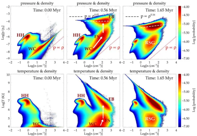
physical mechanisms co-exist. In this section, we discuss the evo-lution of the phase space of the ISM under the influence of the jet is depicted in Fig.12. This figure depicts the 2D mass-weighted PDF3_of_p_versus_ρ _and_T_versus_{ρ. A mass-weighted PDF gives}

preferential weights to the dense gas and hence is a more effective probe of the denser ISM than a volume-weighted analysis. Table4

summarizes the different phases and their labels. Att₌0, the sim-ulation domain has a two phase ISM consisting of a low-density HH and a warm dense turbulent filamentary medium (WC) atT_∼ 104_{K near the central}

∼2 kpc (see Fig.1). Efficient atomic

cool-ing renders the turbulent filaments nearly isothermal as the ISM is allowed to settle prior to the injection of the jet.

With the onset of the jet, two other phases are clearly discernible. At first, a fast-moving forward shock sweeps through the ISM (as shown in Fig.6) shocking the gas to_∼105_{K. The ISM shocked by}

the forward shock is labelled ‘FS’ in Fig.12. The forward shock is followed by a slower, nearly adiabatically expanding high-pressure energy bubble withT _∼ 106–107K. (labelled ‘EB’ in Fig. 12). The energy bubble is nearly homogeneous in pressure and depends only weakly on density as shown by the fits (white dashed lines in Fig.12) to the mean pressure–density relationship of this phase. At later times, the effective polytropic index of the ISM in the bubble increases slightly as the pressure inside the bubble weakens and the denser filaments start to cool. After the jet has broken out and decoupled from the turbulent ISM (t1.33 Myr, corresponding to the third row of Fig.12), there still remains a fraction of the gas shocked at_∼105_{K (RSG). This corresponds to the dense cores of}

the filaments which having survived shredding by the energy bubble have started to cool.

(ii) Polytropic turbulence:

in Fig.13, we show the 2D PDF ofMversus ρ, whereMis the mach number defined byM₌v/cs,csbeing the sound speed.

For the settling ISM, the dense filaments form a region of isother-mal supersonic turbulence (left-hand panel of Fig.13). The Mach number is only weakly correlated with the density, similar to pre-viously reported results from numerical simulations of supersonic isothermal turbulence (Kritsuk et al.2007; Federrath et al.2010; Federrath & Banerjee2015). Ideally for isothermal supersonic tur-bulence, the mach number is independent of the density if the density fluctuations are completely random at all scales (Passot & V´azquez-Semadeni1998). The weak correlations appearing in

3_{The mass-weighted PDFs are constructed by evaluating a 2D histogram of}

a quantity and counting the mass in each simulation cell normalized to the total mass as the weights for a histogram bin.

the numerical simulations result from strong shocks or rarefactions, where the fundamental assumptions of the independence of the density fluctuations break down (Vazquez-Semadeni1994; Passot & V´azquez-Semadeni1998; Federrath et al.2010). With the onset of the jet,M_andρare seen to be positively correlated with density. This is indicative of polytropic turbulence in a medium with poly-tropic index less than unity (Passot & V´azquez-Semadeni1998; Federrath & Banerjee2015), where the PDF deviates from a log-normal distribution.

(iii) Outflow velocity of different phases:

Fig.14shows the temperature versus radial velocity (_|vr|) and

den-sity versus radial velocity (_|vr_|) 2D probability density. We see that

the passage of the forward shock results in heating up of the ISM to∼105_{K as mentioned above without any appreciable increase in}

radial velocity. The clouds are primarily accelerated by the high-pressure energy bubble to speeds of500 kms−1_{. In the right-hand}

panels, we see a tail of very high velocity1000 kms−1_{with less}

mass weight. This corresponds to the low-density cloud ablated ma-terial swept up by the energy bubble to high radial speeds, as shown in Fig.5.

5 D E P E N D E N C E O F M O R P H O L O G Y O N J E T P OW E R

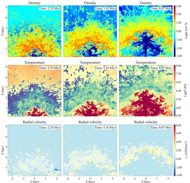
The coupling of the jet with the ISM depends significantly on the jet power. Jets with higher power, although more efficient in driving powerful outflows, drill through the ISM more rapidly causing less shredding of the cloud cores situated a kiloparsec away from the jet axis. Low-power jets, on the other hand, remain trapped in the ISM for a longer time (see Fig.15), interacting with the ISM over a much larger volume. In Fig.16, where we compare the density for jets of different power at a time when the jet head is approximately at the same height for left-hand and right-hand panels. Jets with a power

∼1045ergs−1_{evacuate a central cavity of radius}

∼0.5 kpc, whereas

simulation C withPjet=1044ergs−1a larger cavity (r∼1 kpc) is

evacuated. The situation is more marked for simulation D withPjet=

1043_ergs−1_{, where a larger central cavity is evacuated leaving only}

a few of the densest cores. The density PDFs of the simulation snap-shots in Fig.16are presented in Fig.17. The coefficients of the fits to the high density portion of the density PDF following equation (A7) is presented in Table5. For simulations with low-power jets, the mean density and dispersion of the density PDF is less than half of their counterparts withPjet=1045ergs−1. This indicates more

shredding of the dense cores by the trapped energy bubble. The evolution of the phase space is also significantly different for simulation D, as shown in Fig.18. Unlike the high-power jets, the phase space of the ISM cannot be distinctly divided into a high-pressure energy bubble and gas shocked by the forward shock. The energy bubble is depicted by a horizontal branch in the left-hand panel of Fig.18. Comparing with the left-hand panel of Fig.12

depicting the initial condition of the ISM before the jet injection, we find the bubble for Sim. D to be very weakly overpressured. Slow evolution of the bubble facilitates cooling of the shocked gas. Most of the gas swept up by the bubble is shocked toT_∼105–106K, lower than that of the high-power jets. The weak bubble is unable to accelerate the clouds to high velocities (as shown in the right-hand panel of Fig.18). Thus, although the bubble is weak and does not drive significant outflows apparently indicative of weak feedback, its effect on the density distribution is significant, since it is trapped for a longer time inside the ISM.

(11)

Figure 12. Top: mass-weighted 2D PDF of pressure versus density at times corresponding to plots in Fig.5.p0=9.2×10−4_{dynes cm}−2_{is the scale pressure} of the simulation. The colour bar denotes the probability. The red dotted line for an isothermal gas is presented to highlight that dense gas closely approximates

an isothermal distribution att=0. The white dashed line represents fits to the mean pressure for the phase corresponding to the energy bubble. The pressure

is only weakly related to the density for this phase. Bottom: mass-weighted 2D PDF of temperature versus density. The different ISM phases are labelled as

described in Table4.

Table 4. Summary of different ISM phases.

Phase Description Characteristics

acronym

HH Hot Halo The ambient low-density hot halo. Temperature:T∼107_K.

WC Warm clouds Turbulent warm (T∼104K) dense filaments

describing the initial ISM.

FS Forward shock Shocked ISM behind the initial forward shock. Temperature:T∼105_K.

Very little acceleration from initial turbulent velocity.

EB Energy bubble High-pressure energy bubble expanding nearly adiabatically

forPjet1044ergs−1. Temperature:T∼106–107K.

Accelerates clouds to outward radial velocities500 kms−1

RSG Remnant shocked gas ISM shocked by the forward shock which remains after jet

has decoupled. These represent cooling dense cores of the clouds.

6 E N E R G E T I C S O F T H E J E T- D I S T U R B E D I S M

6.1 Kinetic energy imparted to the ISM

For any jet power, the jet couples strongly with the ISM initially as it drills through the dense medium. Fig.19shows the evolution of the kinetic energy of the dense ISM (ρ >1 cm−3_{) for different}

simulations. The kinetic energy rises with time and then decreases after the jet breaks out and decouples from the ISM. For a jet of power _∼1045_ergs−1_{, the kinetic energy of the ISM increases by}

a factor of 6 or more, whereas forPjet∼ 1044 ergs−1the kinetic

energy increases by a factor of 3. The efficiency of jet feedback is

better illustrated by plotting the ratio of the kinetic energy of the medium to the total integrated energy input of the jet as a function of time (lower panel in Fig.19). We see that_∼25–30 per cent of the jet energy is injected into the ISM, for jets of power1044_ergs−1_.

This is similar to the previous results of (O’Neill et al. (2005), Gaibler et al. (2009),WBU12and Hardcastle & Krause (2013), where initially the jet is shown to impart∼20–30 per cent of its energy as kinetic energy to the ISM, while the rest is deposited as internal energy, a fraction of which will be radiated away. More detailed analysis of the energy budget will be presented in a future work.

(12)

Figure 13. Mass-weighted 2D PDF of log(M) versus log (ρ) at times corresponding to plots in Fig.5. The dashed line represents fits to the mean pressure.

Figure 14. Mass-weighted 2D PDF of temperature versus radial velocity (top) and density versus radial velocity (bottom) at times corresponding to plots in

Fig.5. After the jet injection, the warm dense medium is shocked to∼105_{K by the forward shock without an appreciable increase in velocity. Dense gas is}

accelerated to radial velocities500 kms−1_{by the hot pressure bubble.}

The evolution of the kinetic energy is however very different for a low-power jet as in Sim. D withPjet =1043 ergs−1, due to

the weakly overpressured nature of the bubble. Although the jet strongly interacts with the ISM in its immediate surroundings, the total kinetic energy of the ISM decreases with time. This is because the jet evolves very slowly and at the initial stages the outer layers of the turbulent ISM are not affected. Even at later stages, since the weakly overpressured bubble evolves very slowly, the bulk kinetic energy of the gas decreases as a result of atomic cooling. Thus, simply computing the ratio of the total kinetic energy of the ISM to the energy injected by the jet as an indicator of the effect of feedback of the jet on the ISM is misleading in this case. The effect of the jet on the density PDF is a better probe of jet-ISM coupling for such cases.

6.2 Galactic fountains and the effect on star formation

Although the high-power jets (Pjet1045ergs−1) launch very fast

outflows with speeds500 kms−1_{, the fraction of total mass ejected}

from the influence of the galaxy’s potential is small. In Fig.20, we show the maximum radial distance the accelerated gas may reach by assuming a ballistic trajectory for the gas and solving φ(rmax)−φ(r0)=v02/2, for the maximum radius rmax, wherer0

andv0are the initial radius and radial velocity, respectively. In this

way, we estimate the fractional mass of the ISM that will reach a given distance. The escape fraction is computed after the jet break out when the jet has decoupled from the ISM and the kinetic energy of the ISM saturates as shown in Fig.19. We see that only a small fraction of the gas (5 per cent) goes beyond 10 kpc. Simulation B

(13)

Figure 15. Evolution of density (in cm−3_{), temperature (in Kelvin) and radial velocity (normalized to 100 kms}−1_{) for Sim. D with}_P

jet=1043ergs−1_{. The}

jet remains trapped in the ISM for a much longer time as compared to jets of higher power. The trapped energy bubble affects a larger volume of the ISM.

with lower initial mean density has a larger fraction of mass ejected, as the less dense gas is easier to accelerate. ForPjet=1043ergs−1,

all of the gas is retained within_∼5 kpc. This indicates that although powerful jets can launch fast outflows, the fractional mass-loss is very small and is slightly higher for an ISM with lower mean density. The implication of this result is that the gas is not completely dispersed even though it is accelerated to a radial speed exceeding the velocity dispersion. Instead it forms a galactic fountain in which the gas eventually falls back into the central regions of the galaxy. There may be a temporary inhibition of star formation as a result of the driving of gas out to a few kpc and the production of turbu-lence. Thus, turbulent kinetic energy injected by the jet is probably a more important regulator of star formation activity than mass-loss by outflows, as also reported recently in the observational papers by Lanz et al. (2015a) and Alatalo et al. (2015). We have calculated the mean velocity dispersion in our simulations by computing the variance of the three velocity components from adjacent cubes of dimensions 5_×5_×5 cells in the simulation domain. The jet-driven energy bubble significantly increases the turbulent velocity disper-sion of the swept-up gas, as shown in Fig.21. The mass in the

swept-up shell is seen to have significantly high-velocity dispersion indi-cating the existence of strong turbulent motions, which can signifi-cantly affect star formation (Krumholz & McKee2005; Federrath & Klessen2012). Detailed quantitative analysis of the effect of jets on the star formation rate in the host galaxy will be addressed in a future work.

7 S U M M A R Y A N D D I S C U S S I O N

Let us now summarize the main results from this work as follows.

(i) Filamentary nature of settling ISM:

the simulations of the settling, turbulent ISM result in elongated filaments of dense gas, rather than spheroidal clouds. The fila-ments are caused by shearing of dense clouds and turbulent mixing; this feature is also seen in simulations of driven turbulence (see Federrath & Klessen2012; Federrath & Banerjee 2015, and ref-erences therein). Recent observations with high spatial resolution of high-redshift galaxies also report a filamentary nature of the

(14)

Figure 16. Density (in cm−3_{) at the}_x_–_z_{plane for different simulations. Upper panel: jets of power 10}45_{erg s}−1_{(left, Sim. A) and 10}43_{erg s}−1_{(right, Sim.}

D) passing through the same initial ISM derived from a relaxed turbulent fractal withnw0=300 cm−3_{(see Sections 2.2 and 3 for details). Lower panels: jets}

of power 1045_{erg s}−1_{(left, Sim. B) and 10}44_{erg s}−1_{(right, Sim. C), for an ISM initialized with}_n

w0∼150 cm−3_.

Figure 17. The density PDF of the ISM of simulations corresponding to

Fig.16. The PDF of the ISM before the injection of the jet is represented

in black. The jets of lower power are more effective in destroying the high-density cloud cores.

Table 5. Coefficients of the fit to the density PDF in Fig.16. Sim. A, D

No. Parameter t=0 P45 P45/100

1 ρ¯in cm−3 _21.38 _16.51 ₇

2 σρin cm−3 52.68 31.27 9.32

3 η 0.14 0.11 0.37

4 ρ˜>in cm−3 50 35.54 20.19

Sim. B, C

No. Parameter t=0 P45 P45/10

1 ρ¯in cm−3 12.32 9.17 3.98

2 σρin cm−3 24.74 15.88 7.52

3 η 0.19 0.15 0.28

4 ρ˜>in cm−3 34.2 26.63 21

Note.P45=Pjet=1045ergs−1

extended halo of gas (Swinbank et al. 2015a,b; Wisotzki et al.

2016). After_∼2 Myr, corresponding approximately to half the dy-namical time_∼rB/σB, the filaments settle to form a turbulent central

region of warm gas (T_∼104_{K) extending to about}

∼2 kpc and

an HH (T_∼107K). Fig.3shows the volume filling factor of the ISM, with the dense gas (n > 10 cm−3_{) having a filling factor} 0.1.

(ii) Evolution of the energy bubble and multiphase ISM: the jet launches a high-pressure energy bubble, which sweeps through the ISM. The bubble is preceded by a forward shock, which heats the filaments to temperatures_∼105 _{K but does not}

(15)

Figure 18. 2D PDF for Sim. D withPjet=1043_ergs−1_at_∼_{9 Myr. The evolution of the ISM is significantly different from that of the high-power jets, as}

inferred by comparing similar plots presented in Figs12–14. A significant amount of the gas remains in the mildly hot phase (∼105_{k) from the forward shock.}

The temperature–velocity plot shows very little outward radial acceleration of the gas.

Figure 19. The evolution of the kinetic energy of the dense ISM (ρ >1

cm−3_{) with time. The top panel shows the fractional increase of the kinetic}

energy of the ISM from its initial value. The lower panel plots the kinetic energy at a given time normalized to the total energy injected by jet till that time, indicating the efficiency of coupling of the jet.

accelerate them (Fig.14). The high-pressure energy bubble pro-gresses more slowly, shearing and accelerating the filamentary fragments, creating fast radial outflows (_∼500 kms−1 _for _P

jet =

1045_ergs−1_{). The shocks driven by the energy bubble create a}

mul-tiphase ISM of mildly hot (T_∼105K) gas in the outer layer of the forward shock. The forward shock is followed by an adiabatically expanding hot energy bubble (T_∼106–107K). Observational ev-idence of such shocked multiphase ISM have been obtained from extended X-ray emission from radio-loud galaxies (Kraft et al.2003; Croston, Kraft & Hardcastle2007; Mingo et al.2011; Wang et al.

2012). Clouds trapped in the energy bubble are shredded with their outer layers flowing out in fast, hot, low-density outflows (withT> 106_K,_n_<_{10 cm}−3_,_v

r_∼1000 kms−1). The dense central cores are

Figure 20. The figure shows the maximum radial distance a gas with a given velocity may reach under the influence of gravity, expressed as a fraction of the total ISM mass.

radially accelerated to velocities of_∼500 kms−1_{. Such velocities}

are in agreement with observations of jet-driven outflows (see for exampleWBU12; Collet et al.2016, and references therein).

(iii) Feedback from low-power jets:

a significant result from this work is the effect of low-power jets on the ISM of the host galaxy. High-power jets, although more effective in launching faster outflows, are less destructive of the ISM since they efficiently drill through the ISM. Low-power jets lack sufficient momentum to readily pierce the ISM and remain trapped for a longer time. This results in a more lateral spreading of the trapped energy bubble which causes enhanced shearing of the ISM filaments (as shown in Figs16and17). Such persistent coupling of a trapped jet with the ambient ISM will result in constant stirring of the turbulent ISM, inhibiting star formation in the process. This agrees with recent suggestions of suppressed star formation in some systems with a weak radio jet, such as NGC 1266 (Nyland et al.2013; Alatalo et al.

2015) and some molecular hydrogen emission galaxies with weak radio jets (Ogle et al.2007,2010; Lanz et al.2015a).

As noted in Section 1, the radio luminosity function implies that the distribution of 1.4 GHz radio power,P1.4, peaks at around the

FRI/FRII break at 1024.6_{W Hz}−1_{(Mauch & Sadler}₂₀₀₇_).

Approx-imately this corresponds toPjet∼1042−43erg s−1. Thus, given our

results from the simulation withPjet=1043erg s−1, we expect that

low-powered jets withPjet1043erg s−1should play a significant

role in affecting the evolution of the ISM and star formation in the host galaxy.

(16)

Figure 21. The velocity dispersion map at thex–zplane for simulation A. The colour bar represents log (σ),σbeing the mean of the dispersion of the three

velocity components (σ2=3_i

=1σ 2

i/3).

(iv) Efficiency of feedback:

the jet significantly couples to the ISM within the central few kpc before it breaks out into the ambient halo. From Fig.19, we see that nearly_∼30 per cent of the jet energy is transferred as kinetic energy to the ISM for high-power jets. This measure of coupling efficiency4

is independent of jet power and density, as long as the jet creates a sufficiently overpressured bubble. This agrees with previous results ofWBU12.

(v) Small net mass-loss:

only a few per cent of the dense gas mass is ejected from the galaxy to large distances (see Fig.20). Most of the mass affected by the energy bubble is expected to rain back down into the galaxy’s potential on free-fall time-scales – typically of the order of a few tens of Myr. This supports the galactic fountain scenario of jet-driven feedback (similar to Oppenheimer et al.2010; Dav´e et al.

2012). The jets may cause temporary quenching of star formation by launching local outflows and making the ISM turbulent, but the ejected mass will fall back and may be available for star formation after a few tens of Myr. The effect of such repeated cyclic explosive episodes and its connection to the AGN duty cycle needs to be explored in future work.

AC K N OW L E D G E M E N T S

This research was supported by the Australian Research Council through the Discovery Project, The Key Role of Black Holes in Galaxy Evolution, DP140103341. We thank Christoph Federrath, Matt Lehnert and Nicole Nesvadba for useful discussions. We thank the HPC and IT teams at the National Computational Infrastructure, the ANU, the Pawsey Supercomputing Centre and RSAA for their help and support in carrying out the simulations and subsequent analysis. We acknowledge constructive comments by the referee, which assisted us in improving the original manuscript.

R E F E R E N C E S

Alatalo K. et al., 2015, ApJ, 798, 31

Allen S. W., Dunn R. J. H., Fabian A. C., Taylor G. B., Reynolds C. S., 2006, MNRAS, 372, 21

Allen M. G., Groves B. A., Dopita M. A., Sutherland R. S., Kewley L. J., 2008, ApJS, 178, 20

Asplund M., Grevesse N., Sauval A. J., Scott P., 2009, ARA&A, 47, 481

4_E_kin/_P

jett,Ekinbeing the kinetic energy of the dense gas (n>1 cm−3).

Auriemma C., Perola G. C., Ekers R. D., Fanti R., Lari C., Jaffe W. J., Ulrich M. H., 1977, A&A, 57, 41

Best P. N., Kauffmann G., Heckman T. M., Brinchmann J., Charlot S., Ivezi´c ˇZ., White S. D. M., 2005, MNRAS, 362, 25

Bicknell G. V., 1995, ApJS, 101, 29 Binney J., Tabor G., 1995, MNRAS, 276, 663

Bower R. G., Benson A. J., Malbon R., Helly J. C., Frenk C. S., Baugh C. M., Cole S., Lacey C. G., 2006, MNRAS, 370, 645

Castor J., McCray R., Weaver R., 1975, ApJ, 200, L107 Ciotti L., Ostriker J. P., Proga D., 2010, ApJ, 717, 708 Colella P., Woodward P. R., 1984, J. Comput. Phys., 54, 174 Collet C. et al., 2016, A&A, 586, A152

Croston J. H., Kraft R. P., Hardcastle M. J., 2007, ApJ, 660, 191 Croston J. H. et al., 2008, A&A, 487, 431

Croton D. J. et al., 2006, MNRAS, 365, 11

Dasyra K. M., Combes F., Novak G. S., Bremer M., Spinoglio L., Pereira Santaella M., Salom´e P., Falgarone E., 2014, A&A, 565, A46 Dasyra K. M., Bostrom A. C., Combes F., Vlahakis N., 2015, ApJ,

815, 34

Dav´e R., Finlator K., Oppenheimer B. D., 2012, MNRAS, 421, 98 Del Zanna G., Dere K. P., Young P. R., Landi E., Mason H. E., 2015, A&A,

582, A56

Di Matteo T., Springel V., Hernquist L., 2005, Nature, 433, 604 Diehl S., Statler T. S., 2008, ApJ, 687, 986

Dopita M. A., Sutherland R. S., Nicholls D. C., Kewley L. J., Vogt F. P. A., 2013, ApJS, 208, 10

Dubois Y., Pichon C., Devriendt J., Silk J., Haehnelt M., Kimm T., Slyz A., 2013, MNRAS, 428, 2885

Federrath C., 2016, MNRAS, 457, 375

Federrath C., Banerjee S., 2015, MNRAS, 448, 3297 Federrath C., Klessen R. S., 2012, ApJ, 761, 156 Federrath C., Klessen R. S., 2013, ApJ, 763, 51

Federrath C., Roman-Duval J., Klessen R. S., Schmidt W., Mac Low M.-M., 2010, A&A, 512, A81

F¨orster Schreiber N. M. et al., 2009, ApJ, 706, 1364 Gabor J. M., Bournaud F., 2014, MNRAS, 441, 1615

Gaibler V., Krause M., Camenzind M., 2009, MNRAS, 400, 1785 Gaibler V., Khochfar S., Krause M., 2011, MNRAS, 411, 155 Gaibler V., Khochfar S., Krause M., Silk J., 2012, MNRAS, 425, 438 Gaspari M., Ruszkowski M., Sharma P., 2012, ApJ, 746, 94 Godfrey L. E. H., Shabala S. S., 2016, MNRAS, 456, 1172

Goulding A. D. et al., 2016, preprint (arXiv:1604.01764)

Hardcastle M. J., Krause M. G. H., 2013, MNRAS, 430, 174 Hopkins P. F., 2013, MNRAS, 430, 1880

Hopkins P. F., Elvis M., 2010, MNRAS, 401, 7

Hopkins P. F., Torrey P., Faucher-Gigu`ere C.-A., Quataert E., Murray N., 2016, MNRAS, 458, 816

Klessen R. S., 2000, ApJ, 535, 869

Konstandin L., Girichidis P., Federrath C., Klessen R. S., 2012, ApJ, 761, 149

(17)

P., Emonts B. H. C., Oosterloo T. A., 2016, MNRAS, 455, 2453 Mart´ı J. M. l., M¨uller E., 1996, J. Comput. Phys., 123, 1

Mauch T., Sadler E. M., 2007, MNRAS, 375, 931

Maughan B. J., Giles P. A., Randall S. W., Jones C., Forman W. R., 2012, MNRAS, 421, 1583

Mignone A., McKinney J. C., 2007, MNRAS, 378, 1118

Mignone A., Bodo G., Massaglia S., Matsakos T., Tesileanu O., Zanni C., Ferrari A., 2007, ApJS, 170, 228

Mingo B., Hardcastle M. J., Croston J. H., Evans D. A., Hota A., Kharb P., Kraft R. P., 2011, ApJ, 731, 21

Morganti R., Fogasy J., Paragi Z., Oosterloo T., Orienti M., 2013, Science, 341, 1082

Morganti R., Oosterloo T., Oonk J. B. R., Frieswijk W., Tadhunter C., 2015, A&A, 580, A1

Murray N., Quataert E., Thompson T. A., 2005, ApJ, 618, 569

Nesvadba N. P. H., Lehnert M. D., De Breuck C., Gilbert A., van Breugel W., 2007, A&A, 475, 145

Nesvadba N. P. H., Lehnert M. D., De Breuck C., Gilbert A. M., van Breugel W., 2008, A&A, 491, 407

Nesvadba N. P. H., Boulanger F., Lehnert M. D., Guillard P., Salome P., 2011, A&A, 536, L5

Nicholls D. C., Dopita M. A., Sutherland R. S., Kewley L. J., Palay E., 2013, ApJS, 207, 21

Nyland K. et al., 2013, ApJ, 779, 173

O’Neill S. M., Tregillis I. L., Jones T. W., Ryu D., 2005, ApJ, 633, 717 Ogle P., Antonucci R., Appleton P. N., Whysong D., 2007, ApJ,

668, 699

Ogle P., Boulanger F., Guillard P., Evans D. A., Antonucci R., Appleton P. N., Nesvadba N., Leipski C., 2010, ApJ, 724, 1193

Ogle P. M., Lanz L., Appleton P. N., 2014, ApJ, 788, L33

Oppenheimer B. D., Dav´e R., Kereˇs D., Fardal M., Katz N., Kollmeier J. A., Weinberg D. H., 2010, MNRAS, 406, 2325

Padoan P., Jones B. J. T., Nordlund Å. P., 1997, ApJ, 474, 730 Passot T., V´azquez-Semadeni E., 1998, Phys. Rev. E, 58, 4501 Rawlings S., Saunders R., 1991, Nature, 349, 138

Rosen A. L., Lopez L. A., Krumholz M. R., Ramirez-Ruiz E., 2014, MNRAS, 442, 2701

Sadler E. M., Jenkins C. R., Kotanyi C. G., 1989, MNRAS, 240, 591 Sanders R. L. et al., 2016, ApJ, 816, 23

Saxton C. J., Bicknell G. V., Sutherland R. S., Midgley S., 2005, MNRAS, 359, 781

Schawinski K., Thomas D., Sarzi M., Maraston C., Kaviraj S., Joo S.-J., Yi S. K., Silk J., 2007, MNRAS, 382, 1415

Shirazi M., Brinchmann J., Rahmati A., 2014, ApJ, 787, 120 Silk J., Rees M. J., 1998, A&A, 331, L1

Soker N., White R. E., III, David L. P., McNamara B. R., 2001, ApJ, 549, 832

Stone J. M., Ostriker E. C., Gammie C. F., 1998, ApJ, 508, L99 Sutherland R. S., Bicknell G. V., 2007, ApJS, 173, 37 Sutherland R. S., Dopita M. A., 1993, ApJS, 88, 253 Swinbank A. M. et al., 2015a, MNRAS, 449, 1298 Swinbank A. M. et al., 2015b, ApJ, 806, L17

Synge J. L., 1957, The Relativistic Gas. North-Holland Publishing Com-pany, Amsterdam

A P P E N D I X A : P R O B A B I L I T Y D E N S I T Y F U N C T I O N S

The lognormal distribution has proven to provide excellent descrip-tion of the density prPDF for simuladescrip-tions of isothermal turbulence (Li, Klessen & Mac Low2003; Kritsuk et al.2007; Federrath et al.

2010). The distribution is defined as a Gaussian ins₌lnρwith a mean₋σ_s2/2 and varianceσ_s2:

PV(s)₌ 1 σs√2π

exp

−(s+σ 2

s/2)2 2σ2

s

(A1)

The subscriptVrefers to volume-weighted PDF, which is considered primarily in this work while describing the 1D density PDFs. The above definition of the PDF satisfies the following two conditions of normalizations:

∞

−∞

PV(lnρ)d lnρ₌1 (A2)

∞

−∞

ρPV(lnρ)₌ρ˜ (mean density). (A3)

The mean of the distribution is

lnρ_{= −}σ

2

s

2 (A4)

ρ₌ρ¯ (A5)

and the variance inρis

σ_ρ2₌ρ¯2 exp

σ_s2

−1

. (A6)

In the presence of strong shocks, the density PDF shows sig-nificant departure from a true lognormal, especially in the high-and low-density tails. An improved function proposed by Hopkins (2013) gives a better description of the density PDF in the presence of intermittency:

PV(s)₌I1

2 λu(s)exp [_−{λ₊u(s)_}]

λ u(s)η2

u(s)₌ λ 1₊η−

s

η (u≥0) ;s=ln (ρ/ρ)¯

λ₌ σ

2

s

2η2. (A7)

Here,I1is the modified Bessel function of the first kind. The PDF

in equation (A7) is defined by three parameters: the mean density ¯

ρ which is defined by A2, the dispersion (σs) and a parameterη defining the degree of departure from a lognormality. Forη₌0,

(18)

equation (A7) reduces to the standard expression of a lognormal distribution (equation A1). The mean density of the improved func-tion is same as in equafunc-tion (A4) above. The variance inρis given by

σρ2=ρ¯

2_exp σs2 1₊3η₊2η2

−1

. (A8)

A P P E N D I X B : A D I A B AT I C E X PA N S I O N O F A N E N E R G Y B U B B L E

For a spherical bubble with radius RB, expanding with uniform

pressure (pB), driven by a constant input energy flux from a jet or

wind (Pj), the energy equation can be written as

d dt

₄_π

3 pB

γ₋1R

3 B

+4πR_B2p_BdRB

dt =Pj−Lcool (B1)

d dt

pBR3γ= 3(γ−1)

4π

PjR3(_Bγ−1), (B2)

whereγis the adiabatic index andLcoolis energy loss from atomic

cooling. The first term in the left hand side of equation (B1) is the change of internal energy inside the volume, while the second term is the work done by the expanding bubble. Since we are considering

an adiabatically expanding bubble, we do not consider the cooling losses in equation (B2). If the radius expands asRB∝tα, following

equation (B2), we find that the pressure to evolve as

pB∝t1−3α. (B3)

For a self-similarly expanding bubble in an ISM of constant density (ρ0), the radius and pressure evolve as (Castor et al.1975; Weaver

et al.1977)

RB_∝

Pj ρ0

1/5

t3/5; pB_∝t−4/5. (B4)

However, in a multiphase ISM the bubble expansion is slower than the adiabatic case due to cooling losses and turbulent mixing (e.g. Rosen et al.2014). For Fig.11, we find the radius to evolve asRB∝

t0.55. For an adiabatically expanding bubble, this implies (following equation B3) that the pressure should vary aspB ∝ t−0.65. This

approximately agrees with the initial evolution of the mean pressure of the bubble (shown in Fig.10), for the simulations with high-power jets (Pjet 1044ergs−1). This indicates that for jets with higher

power, an overpressured bubble is formed which initially evolves as an adiabatically expanding spherical bubble till jet break out.

This paper has been typeset from a TEX/LA_{TEX file prepared by the author.}