t uni ng i n r educ i ng bi as es of t op- of - at m
os pher e
r adi at i on and c l ouds i n M
I RO
C ver s i on 5
著者
O
gur a Tom
oo, Shi ogam
a H
i deo, W
at anabe
M
as ahi r o, Yos hi m
or i M
as akaz u, Yokohat a Tokut a,
Annan J am
es D
. , H
ar gr eaves J ul i a C. , U
s hi gam
i
N
aot o, H
i r ot a Kaz uya, Som
eya Yu, Kam
ae
Youi c hi , Tat ebe H
i r oaki , Ki m
ot o M
as ahi de
j our nal or
publ i c at i on t i t l e
G
eos c i ent i f i c m
odel devel opm
ent
vol um
e
10
num
ber
12
page r ange
4647- 4664
year
2017- 12
権利
( C) Aut hor ( s ) 2017.
Thi s w
or k i s di s t r i but ed under t he Cr eat i ve
Com
m
ons At t r i but i on 3. 0 Li c ens e.
U
RL
ht t p: / / hdl . handl e. net / 2241/ 00150613
https://doi.org/10.5194/gmd-10-4647-2017 © Author(s) 2017. This work is distributed under the Creative Commons Attribution 3.0 License.
Effectiveness and limitations of parameter tuning in reducing biases
of top-of-atmosphere radiation and clouds in MIROC version 5
Tomoo Ogura1, Hideo Shiogama1, Masahiro Watanabe2, Masakazu Yoshimori3, Tokuta Yokohata1, James D. Annan4, Julia C. Hargreaves4, Naoto Ushigami5, Kazuya Hirota2, Yu Someya2, Youichi Kamae6, Hiroaki Tatebe7, and
Masahide Kimoto2
1National Institute for Environmental Studies, Tsukuba, Ibaraki, Japan
2Atmosphere and Ocean Research Institute, University of Tokyo, Kashiwa, Chiba, Japan
3Faculty of Environmental Earth Science, Global Institution for Collaborative Research and Education, and Arctic Research
Center, Hokkaido University, Sapporo, Hokkaido, Japan
4BlueSkiesResearch.org.uk, Settle, North Yorkshire, UK
5Graduate School of Life and Environmental Sciences, University of Tsukuba, Tsukuba, Ibaraki, Japan 6Faculty of Life and Environmental Sciences, University of Tsukuba, Tsukuba, Ibaraki, Japan
7Japan Agency for Marine-Earth Science and Technology, Yokohama, Kanagawa, Japan
Correspondence:Tomoo Ogura ([email protected])
Received: 10 May 2017 – Discussion started: 21 June 2017
Revised: 27 October 2017 – Accepted: 9 November 2017 – Published: 21 December 2017
Abstract. This study discusses how much of the biases in top-of-atmosphere (TOA) radiation and clouds can be re-moved by parameter tuning in the present-day simulation of a climate model in the Coupled Model Inter-comparison Project phase 5 (CMIP5) generation. We used output of a perturbed parameter ensemble (PPE) experiment con-ducted with an atmosphere–ocean general circulation model (AOGCM) without flux adjustment. The Model for Inter-disciplinary Research on Climate version 5 (MIROC5) was used for the PPE experiment. Output of the PPE was com-pared with satellite observation data to evaluate the model biases and the parametric uncertainty of the biases with re-spect to TOA radiation and clouds. The results indicate that removing or changing the sign of the biases by parameter tuning alone is difficult. In particular, the cooling bias of the shortwave cloud radiative effect at low latitudes could not be removed, neither in the zonal mean nor at each latitude– longitude grid point. The bias was related to the overestima-tion of both cloud amount and cloud optical thickness, which could not be removed by the parameter tuning either. How-ever, they could be alleviated by tuning parameters such as the maximum cumulus updraft velocity at the cloud base. On the other hand, the bias of the shortwave cloud radiative ef-fect in the Arctic was sensitive to parameter tuning. It could
be removed by tuning such parameters as albedo of ice and snow both in the zonal mean and at each grid point. The ob-tained results illustrate the benefit of PPE experiments which provide useful information regarding effectiveness and limi-tations of parameter tuning. Implementing a shallow convec-tion parameterizaconvec-tion is suggested as a potential measure to alleviate the biases in radiation and clouds.
1 Introduction
re-gions (Nam et al., 2012; Bodas-Salcedo et al., 2014). Previ-ous studies suggest that such biases in radiation and clouds might affect the simulated climate in remote regions or dis-tort the cloud feedback in future projections (Trenberth and Fasullo, 2010; Ceppi et al., 2012). Therefore, alleviating the biases by developing climate models is important.
There are two factors which might contribute to the biases in climate simulated by the models: (a) inappropriate model structures, namely, equations representing the physical pro-cesses or spatial resolution of the model; and (b) inappro-priate parameter values, which are specified in the equations. We therefore attempt to alleviate the biases by modifying fac-tors (a) and (b) within the plausible range during the model development process.
How much of the existing biases can be explained by the second factor (b)? In other words, how much of the biases can be removed by modifying only specified parameter val-ues (parameter tuning)? This issue is important when dis-cussing the model development strategy because it helps to decide which factor, (a) or (b), should be given a priority to efficiently reduce the biases. If the biases in question can be completely explained by factor (b), the priority for parame-ter tuning would be high. In this case, removing the biases is relatively simple because parameter tuning is generally much easier than modifying the model structures. By contrast, if most of the biases cannot be explained by factor (b), modify-ing model structures should be given a high priority.
A perturbed parameter ensemble (PPE) experiment with a climate model is useful when discussing the above issue. In the PPE experiment, we can create different versions of a climate model in a systematic and comprehensive way by modifying the specified parameter values in the model within a plausible range (Murphy et al., 2004). If we evaluate the biases by comparing present-day climate with observation data in each version of the PPE models, we should be able to evaluate parametric uncertainty, namely, the inter-model difference of the biases due to parameter settings. This inter-model difference would also provide a measure regarding how much of the biases can be removed by parameter tun-ing only.
The benefit of PPE experiments, as discussed above, has been illustrated in previous studies. For example, Zhang et al. (2012) conducted a PPE experiment with an atmosphere general circulation model (AGCM) and evaluated the per-formance of cloud simulations compared with satellite ob-servations over various tropical regions. The results indicate that the model performance in simulating clouds is sensi-tive to parameter tuning. Yokohata et al. (2012) focused on different PPE experiments conducted with an atmosphere– ocean GCM (AOGCM), two atmosphere–slab ocean GCMs (ASGCMs), and an AGCM, and evaluated the model perfor-mance in simulating the cloud radiative effect at TOA com-pared with observations. They found that the sensitivity of the model biases to parameter tuning varies widely among different regions. In the PPEs analyzed in the study,
how-ever, the sea surface temperature (SST) bias was suppressed by applying flux adjustment at the sea surface in both the AOGCM and ASGCM.
In the present study, we attempt to better understand the parametric uncertainty of TOA radiation and cloud bi-ases by using the PPE output of an AOGCM without flux adjustment. There is an advantage in using the AOGCM without flux adjustment because climate projections in the CMIP5 Multi-Model Ensemble (MME) are conducted with AOGCMs without flux adjustment and the biases of such AOGCMs are therefore directly relevant for future projec-tions using CMIP5 (Flato et al., 2013). If we suppress the SST biases in the AOGCMs by applying flux adjustment, the TOA radiation and cloud biases in which we are interested might be obscured. In addition, the parametric uncertainty of the biases might be overestimated if we apply flux adjust-ment because it allows us to include AOGCMs with large radiative imbalance at the TOA as valid samples in the PPE, while such models are not used for future projections in the CMIP5 MME.
When evaluating biases in the simulated clouds, we use output of the Cloud Feedback Model Inter-comparison Project (CFMIP) Observation Simulator Package (COSP), which is incorporated into the AOGCM. The COSP is di-agnostic software that processes the GCM outputs, such as the cloud amount, and simulates the signals that would be re-trieved by satellites (Bodas-Salcedo et al., 2011). It increases the chances that the difference between the model output and observation reflects real biases in the model simulation rather than observational limitations. Therefore, COSP has been widely used in previous studies, which evaluate clouds simulated by the CMIP5 MME. The studies indicate that the optical thickness of the simulated clouds tends to be over-estimated compared with the observation, as in the CMIP3 (Klein et al., 2013; Nam et al., 2012; Zhang et al., 2005). In the present study, we evaluate the parametric uncertainty of this too thick (bright) bias by analyzing the COSP output of the PPE experiment, and discuss how much of the bias can be removed by parameter tuning only.
2 Models and methods
2.1 Design of the perturbed parameter ensemble
We compared the output of the PPE experiment using the AOGCM in the pre-industrial control setting with the obser-vation to evaluate the model biases. We used the Model for Inter-disciplinary Research on Climate version 5 (MIROC5) AOGCM. The atmospheric component has a horizontal res-olution of T42 (∼2.8◦) with 40 vertical levels. The ocean
component is COCO4.5 with a horizontal resolution of∼1◦
and 49 vertical levels in addition to a bottom boundary layer. The model is the low-resolution version of the MIROC5 AOGCM, which is used in CMIP5 with a higher resolution of T85 (∼1.4◦) in the atmosphere (Watanabe et al., 2010). We
confirmed that the low-resolution version ran stably and did not suffer from significant climate drift in the pre-industrial control experiment without flux adjustment when the stan-dard setting of the tuning parameters was specified. The model could also reproduce the characteristic biases of the TOA radiation and clouds of the T85 version used in CMIP5. The cloud parameterization of MIROC5 employs a statis-tical scheme. We assume that there is small-scale fluctuation of total water Qt within the model grid box, which is
de-scribed by a probability density function (PDF),G(Qt). We
also assume that the Qt exceeding supersaturation with
re-spect to liquid,Qs, takes the form of cloud liquid. Then the
cloud coverCand cloud liquid contentQcare diagnosed as
the integral over the saturated part of the grid box, as follows:
C=
Z ∞
Qs
G (Qt)dQt, (1)
and
Qc=
Z ∞
Qs
(Qt−Qs)·G (Qt)dQt. (2)
Overbar denotes average over the grid box. The shape of the PDF is represented by a triangular function. The model pre-dicts variance and skewness of the PDF, which are affected by cumulus convection, cloud microphysics, turbulent mix-ing, and advection. Details of the cloud parameterization are described by Watanabe et al. (2009).
MIROC5 also uses a cloud microphysics parameterization following Wilson and Ballard (1999). The parameterization predicts ice water content using physically based tendency terms which represent nucleation, deposition and sublima-tion, riming, and ice melting, among others.
We should note that perturbing specified values of tun-ing parameters might increase the net radiation imbalance at TOA when conducting PPE with an AOGCM in the pre-industrial control setting, which leads to a gradual change in climate different from the initial state (climate drift). Such a change would make the definition of the control climate dif-ficult. In addition, the simulated climate might not be a valid
example of pre-industrial control simulations. Applying flux adjustment at the sea surface would help to suppress the cli-mate drift by reducing the SST biases. However, it might also cover up the biases in the TOA radiation and clouds, which are sensitive to the SST. What we need here is both stable climate and SST biases, as indicated in the CMIP5 pre-industrial control experiments. Therefore, we used the output of the PPE experiment conducted in Shiogama et al. (2012), following the suppressed imbalance sampling (SIS) method, in the present study. The SIS is a method to subsample mem-bers of the PPE with a small imbalance in the TOA radiation and thus with small climate drift. This enables us to study stable climates of the PPE without applying flux adjustment. Other methods analogous to the SIS have been discussed in Jackson et al. (2012) and Yamazaki et al. (2013).
The details of the SIS method are described in Shiogama et al. (2012). For reference, we also present the summary in the following. First, we select 10 tuning parameters, which are considered important to the radiative forcing of CO2
dou-bling, climate feedback, and climate sensitivity (Table 1). The selection is based on the results of sensitivity experi-ments using the atmospheric component of MIROC5, which shows that perturbing the 10 parameters has a large impact on the radiative forcing and climate feedback compared to other tuning parameters. The selected 10 parameters are related to cumulus convection, cloud, turbulence, aerosol, and land sur-face processes. The maximum and minimum values of the parameters are determined by expert judgement so that the parameters are within the plausible range, namely, they are consistent with the observation and current understanding of the climate system. Values of the 10 parameters are then se-lected from the maximum to minimum ranges and randomly paired to produce 5000 samples of 10-D vectors, following Latin hypercube sampling. Each vector corresponds to a set of input values for the 10 tuning parameters. We further se-lect 56 members from the 5000 samples so that the TOA ra-diative imbalance of the selected members is close to that of the standard model. The selection of the 56 members is con-ducted with the following three steps: (1) we conduct a PPE experiment with the MIROC5 AGCM under pre-industrial conditions, in which tuning parameters are changed one at a time to the minimum and maximum values before run-ning the AGCM for 6 years, (2) outputs of the PPE members are linearly interpolated to estimate the TOA radiative im-balance for the 5000 samples of the tuning parameters, and finally, (3) we select 56 members in which the TOA radia-tive imbalance is close to that of the standard model. The number of subsampled members, namely 56, is determined by the computational resources available. Note that the num-ber increased from 35 in the previous study by Shiogama et al. (2012). Finally, we create 56 members of the MIROC5 AOGCM by specifying different members of the 10-D vec-tors for the model as input values for the tuning parameters.
Table 1.List of physics parameters that were varied in the MIROC5 PPE.
Name Category Description Standard Min Max
wcbmaxa Cumulus Maximum cumulus updraft velocity at cloud base (m s−1
) 1.7 0.7 2.8 precz0a Cumulus Base height for cumulus precipitation (m) 500 200 1000 clmda Cumulus Entrainment efficiency (ND) 0.51 0.4 0.6 vicecb Cloud Factor for ice falling speed (m0.474s−1
) 38 25 40
b1c Cloud Berry parameter (m3kg−1
) 0.09 0.07 0.11
faz1d Turbulence Factor for PBL overshooting (ND) 1.5 1 3 alp1d Turbulence Factor for length scaleLT(ND) 0.23 0.16 0.3
tnuwc Aerosol Timescale for nucleation (s) 18 000 14 400 21 600 ucminc Aerosol Minimum cloud droplet number (liquid) (m−3
) 2.5×10⁷ 2.2×10⁷ 3.0×10⁷ albe Surface Albedo of ice and snowf Medium Low High
aChikira and Sugiyama (2010).bWilson and Ballard (1999).cTakemura et al. (2005, 2009).dNakanishi and Niino (2004).eTakata et al. (2003) and Watanabe et
al. (2010).f“alb” indicates a collection of eight parameters corresponding to the albedo of ice and snow over sea and land.
Table 2.Observation data used for the model evaluation. All data are monthly means.
Variable Dataset Period References
Top-of-atmosphere CERES-EBAF (Edition 4.0) March 2000–January 2017 Loeb et al. (2009) radiative fluxes ERBE-S9 January 1985–December 1989 Barkstrom (1984) ISCCP-FD January 1986–December 1990 Zhang et al. (2004)
Cloud fraction GCM simulator-oriented ISCCP cloud product July 1983–June 2008 Pincus et al. (2012), Rossow et al. (1996) CALIPSO-GOCCP June 2006–December 2010 Chepfer et al. (2010)
that the changes in the simulated surface air temperature from the initial state (climate drift) were small. This was ex-pected because the TOA radiative imbalance is close to that of the standard model. Years 1–10 of the simulation were considered to be a spin-up period during which the simulated climate adjusted to the modified tuning parameters. The out-put from years 11 to 30 was averaged to make a climatology. The model biases were defined as the difference of the cli-matology from observation data.
The observation data used for the model evaluation orig-inate in the period of 1983–2017 (Table 2). Therefore, the model output from the historical simulation of the same period is appropriate for comparison with the observation. However, conducting the historical simulation requires an ex-tension for more than 150 years after the pre-industrial con-trol simulation of 30 years. This means a more than 6-fold in-crease in computational cost, which we are not able to cover. Therefore, we decided to use the pre-industrial control sim-ulation as a surrogate for the historical simsim-ulation, assuming that the former reproduces the biases in the latter, regarding TOA radiation and clouds. This assumption is supported by other simulation results. For example, we compared biases in the historical simulation with those in the pre-industrial control simulation using MIROC5 with the horizontal reso-lution of T85 (∼1.4◦). We confirmed that the TOA radiation
and cloud biases in the two simulations were similar to each other (not shown).
2.2 Observation data
Table 2 summarizes the observation data which are com-pared with the model output. They all are monthly mean data. We defined the model biases referring to multiple ob-servations, namely three for TOA radiation and two for the cloud amount; therefore, the observation uncertainty can be taken into account. The biases are considered robust if they are commonly seen with respect to multiple observations. The observation data for TOA radiation are derived from CERES-EBAF (Loeb et al., 2009), ERBE-S9 (Barkstrom, 1984), and ISCCP-FD (Zhang et al., 2004). The data for the cloud amount are from the GCM simulator-oriented ISCCP cloud product (Pincus et al., 2012; Rossow et al., 1996) and CALIPSO-GOCCP (Chepfer et al., 2010). The cloud amount data of the ISCCP are custom-built daytime-only monthly averages, which are available from the CFMIP-OBS website (http://climserv.ipsl.polytechnique.fr/cfmip-obs). We first re-ferred to the observation data to calculate the monthly clima-tology for the period in Table 2. We then interpolated the data linearly to the horizontal resolution of T42 and used them to calculate the difference from the model output.
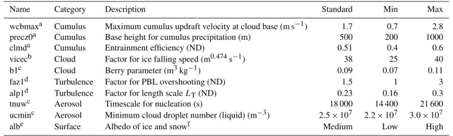
com-Figure 1.TOA radiation bias in the global annual mean for(a)net,(b)longwave and shortwave,(c)longwave clear-sky, shortwave clear-sky, longwave CRE, and shortwave CRE components. The biases are with respect to the average of three observational data, namely, ERBE-S9, ISCCP-FD, and CERES-EBAF. The net radiation of zero with no TOA imbalance is indicated by the dashed line in(a). The unit is W m−2 and the signs are positive downward.
pared the cloud amount identified by the ISCCP simulator with the GCM simulator-oriented ISCCP cloud product and the one determined with the CALIOP lidar simulator with the CALIPSO–GOCCP data. We confirmed that the ISCCP sim-ulator was implemented properly in the MIROC5 AOGCM following Zelinka et al. (2012), which means we calculated the total sum of the cloud amount from the ISCCP simu-lator for all cloud top pressure and optical thickness bins and confirmed that the sum is consistent with the “native” cloud amount identified in the MIROC5 AOGCM. Note that optically thin clouds with TAU<0.3 are not included in this comparison because the available “native” cloud amount does not include such clouds.
3 Parametric uncertainty of the TOA radiation bias
First, we present the outline of the TOA radiation bias of the MIROC5 PPE by discussing the global annual mean values in Fig. 1. The biases in the net radiation are small (Fig. 1a), which means that the values of all PPE members are within the range of the three observations and near the zero net ra-diation with no imbalance, indicated by the dashed line. This was expected because we selected these members when de-signing the PPE following the SIS method. If we focus on the components of the TOA radiation, however, we notice larger biases compared with the net radiation (Fig. 1b, c). The largest biases appear in the SCRE; the biases range from−11.8 to−5.8 W m−2. All PPE members are more than
3.0 W m−2
smaller than either one of the three observations. Therefore, parameter tuning enables us to reduce the bias from −11.8 to−5.8 W m−2 by as much as 50 %; however,
we cannot totally remove it or change its sign. The short-wave clear-sky component (SWclr) also exhibits large biases in which all PPE members are larger than either one of the three observations. Therefore, we cannot change the sign of the bias by parameter tuning only.
We should note that the SCRE biases are negatively cor-related with the LCRE biases with the correlation coefficient of−0.82. Therefore, if we reduce the SCRE bias by making
it more positive, the LCRE bias tends to be more negative.
Figure 2.TOA radiation in the zonal annual mean for the(a) short-wave CRE and(b)longwave CRE components. The unit is W m−2 and the signs are positive downward.
This would reduce the LCRE bias in more than half of the PPE members. Correlations of the SCRE biases with the bi-ases in clear-sky components are small:−0.08 with LWclr
and−0.32 with SWclr.
Next, we discuss the characteristics of the radiation bias on a smaller spatial scale, as shown by the zonal annual mean in Fig. 2. We especially focus on the cloud radiative effect, which illustrates the biases related to clouds. The negative SCRE biases, as observed in the global mean (Fig. 1c), are mostly attributable to the biases at low latitudes (Fig. 2a). At those latitudes, all PPE members are outside the range of the three observations. Therefore, the bias cannot be elim-inated or change sign by parameter tuning, although it can be reduced by∼30 %. In the Arctic, on the other hand, the
inter-model difference among the PPE members tends to be larger compared with other latitudes; hence, the observations lie within the PPE spread. Here, the SCRE bias can be elim-inated or change sign by parameter tuning. The biases of the longwave cloud radiative effect (LCRE) appear to be small at most latitudes (Fig. 2b). At least one of the PPE members is within the range of the three observations at most latitudes.
Figure 3.TOA radiation bias in the annual mean for the(a)shortwave CRE and(b)longwave CRE components. The biases are for the ensemble mean of the MIROC5 PPE with respect to CERES-EBAF. Standard deviation of the TOA radiation bias among the PPE ensemble members for the(c)shortwave CRE and(d)longwave CRE. Fraction of the PPE ensemble members, which have positive signs of the TOA radiation bias, for the(e)shortwave CRE and(f)longwave CRE.
the radiative fluxes more directly than the ISCCP–FD and it also has various advantages over the ERBE–S9 such as scene identification (Wielicki et al., 1996; Loeb et al., 2009). We confirmed that similar results were obtained when using ISCCP–FD or ERBE-S9 (not shown).
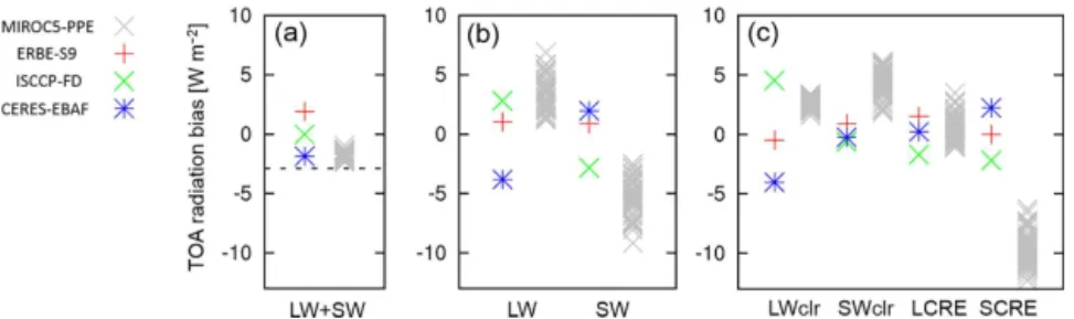
The negative SCRE bias at the low latitudes, as observed in the zonal mean plot (Fig. 2a), appears pronounced over the oceans, exceeding−40 W m−2in large areas (Fig. 3a).
We also notice positive biases at middle to high latitudes over the Southern Ocean, the northwestern part of Eurasia, and the northeastern part of North America. They exceed 5 W m−2
in some places. On the other hand, if we measure the paramet-ric uncertainty of the SCRE bias using the standard devia-tion among the PPE members, we notice that the uncertainty does not exceed 4 W m−2
in most areas (Fig. 3c). Therefore, removing or changing the sign of the SCRE bias at each grid point by parameter tuning only is difficult. This can be con-firmed by the fractions of the PPE members, which have pos-itive biases (Fig. 3e). At each grid point, we count the number of the PPE members which have a positive SCRE bias. Then we divide it by the total number of PPE members, which is
56. The resulting fractions are plotted in Fig. 3e, so that we can see whether the observation data lie within the range of the PPE spread at each grid point. In most areas of the globe, the fraction is 0 (blue) or 1 (orange), which means that obser-vation data are outside the range of the PPE spread, or that all PPE members have the same sign of the SCRE bias. In this case, parameter tuning plays only a limited role in re-ducing the SCRE bias; in particular, the sign of the bias can-not be changed. An exception is the Arctic. Here, the SCRE bias is about 5 W m−2
and the standard deviation of the bias ranges from 6 to 8 W m−2
(Fig. 3a, c). The observation data are within the range of the PPE spread. Therefore, the biases of the PPE members can be either positive or negative, which is indicated by the green and yellow colours in Fig. 3e. Here, we can change the sign of the SCRE bias by parameter tun-ing.
The LCRE bias is smaller than the SCRE bias (Fig. 3a, b). It is smaller than 20 W m−2
in most areas. However, the stan-dard deviation of the LCRE bias is even smaller (Fig. 3d), less than 5 W m−2
Figure 4.Cloud amount bias in the July mean with respect to the(a)CALIPSO and(b)ISCCP observations. The biases are for the ensemble mean of the MIROC5 PPE. Fraction of the PPE ensemble members, which have positive signs of the cloud amount bias, with respect to (c)CALIPSO and(d)ISCCP observation.
most regions except for the northern mid-latitudes and the South Pacific. This is illustrated by the fractions of the PPE members, which have positive biases (Fig. 3f). They are 0 (blue) or 1 (orange) in large areas including the Arctic.
4 Parametric uncertainty of the cloud bias
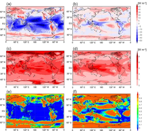
To better understand the origin of the cloud radiative effect bias, we examine the geographical distribution of the cloud amount bias in Fig. 4. In the following, we present results for the boreal summer season when the cloud amount bias is most pronounced in the Hawaiian Trade Cumulus Region, which we discuss later in this section. The cloud amount is overestimated over the Pacific and Atlantic at low latitudes (Fig. 4a, b), which contributes to the negative SCRE bias, as shown in Fig. 3a. The overestimation is a robust feature; it exists with respect to both ISCCP and CALIPSO observa-tions. In addition, all members of the PPE have positive bi-ases in those regions (Fig. 4c, d). Therefore, the bibi-ases can-not be removed by parameter tuning. We should can-note here that the multi-model mean ISCCP cloud amount (TAU>1.3) from the CFMIP1 and CFMIP2 ensembles does not show such positive bias at low latitudes (Klein et al., 2013). There-fore, the bias might be a problem specific to the MIROC5 AOGCM.
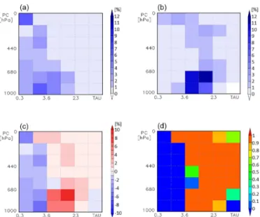
The cloud amount bias can be decomposed into the contri-butions from different cloud top pressure and optical thick-ness bins, as illustrated for the Hawaiian Trade Cumulus Re-gion (15–35◦
N, 160◦ E–140◦
W) in Fig. 5. The region of fo-cus is indicated by the black square in Fig. 4b. The MIROC5
PPE tends to overestimate optically thick clouds (TAU>3.6) and underestimate optically thin clouds (TAU<3.6) com-pared with the ISCCP observation (Fig. 5a, b, c). The con-tribution of the former outweighs that of the latter, which leads to the overestimation of the cloud amount. The over-estimation is especially large in low-top clouds (PC>680). The clouds of the MIROC5 PPE are biased towards optically thick clouds compared with the observation, which also con-tributes to the negative SCRE bias.
We further examined the signs of the cloud biases for each bin of the cloud top pressure and optical thickness categories. The fraction of the positive biases within the PPE members is 0 (blue) or 1 (orange) in 36 out of 42 bins (Fig. 5d); all PPE members have the same cloud bias sign in most (85 %) of the cloud top pressure and optical thickness bins. There-fore, removing the too thick bias by parameter tuning only is considered difficult in this model.
Figure 5.ISCCP cloud amount of the July mean for the Hawaiian Trade Cumulus Region (15–35◦
N, 160◦ E–140◦
W), indicated by the black square in Figure 4b, for different categories of the cloud top pressure (PC) and cloud optical thickness (TAU). Each panel is for(a)ISCCP observation,(b)MIROC5 PPE ensemble mean, (c)model bias, namely(b)minus(a), and (d) fraction of the PPE ensemble members with positive bias.
Figure 6. Relationship between the non-overlapped low cloud amount and shortwave CRE of the July mean for the Hawaiian Trade Cumulus Region.
It is larger by ∼30 W m−2, even if the models have the
same cloud amount as the observation, which indicates that the optical thickness of low-top clouds is overestimated in the MIROC5 PPE. The above-mentioned characteristics are common to all PPE members and the observation is outside the range of the PPE. This again indicates that we cannot re-move the too thick bias by parameter tuning only.
5 Characteristics of different tuning parameters
The results presented so far illustrate the difficulties in re-moving the TOA radiation and cloud biases by parameter tuning. At the same time, however, we also learned that pa-rameter tuning enables us to control the model biases to some extent, demonstrating its benefit for model development. For example, the global mean SCRE bias can be reduced by as much as 50 % by tuning only (Fig. 1c). To obtain the desired effects by parameter tuning, we need to understand the char-acteristics of different tuning parameters. Therefore, in the following, we briefly describe the regions in which the tun-ing parameters in Table 1 control the model biases, focustun-ing on the CRE.
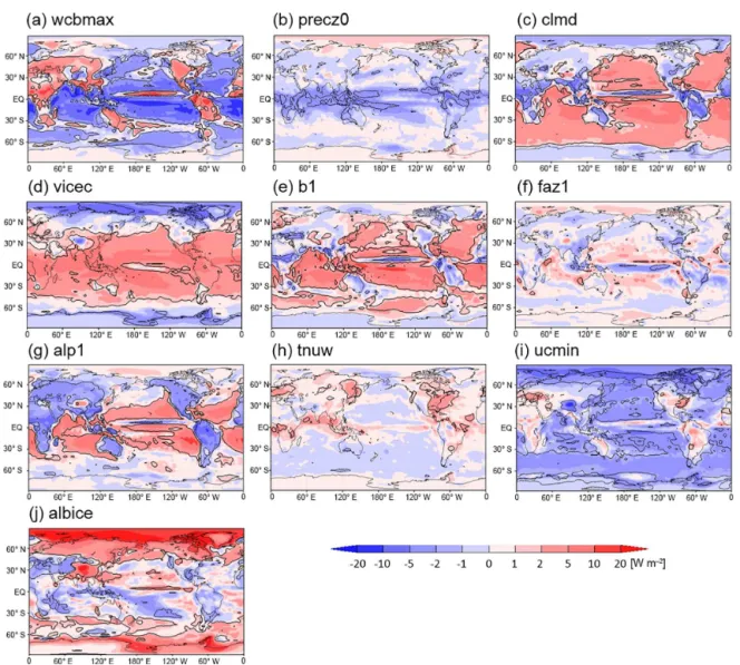
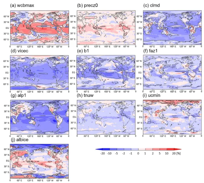
We calculated the regression coefficients of the CRE on different tuning parameters for each latitude–longitude grid point, referring to the 56 members of the PPE, and plotted the geographical distribution of the coefficients in Figs. 7 and 8. In addition, we calculated the regression of the ISCCP cloud properties (cloud amount, cloud optical thickness, and cloud top pressure) on the tuning parameters. The results are shown in Appendix Figs. A1, A2, and A3. Note that the tuning pa-rameters were normalized to the range of 0.0 to 1.0; thus, the coefficients indicate the responses of the CRE and clouds to an increase in the tuning parameters from the minimum to the maximum values in Table 1.
The tuning parameters, which are especially effective in controlling the shortwave CRE, are wcbmax and albice; wcbmax and albice can change the SCRE by more than 10 W m−2
over low-latitude oceans and the Arctic, respec-tively (Fig. 7a, j).
The parameter wcbmax is the maximum cumulus updraft velocity at the cloud base. Increasing the parameter leads to an increase in the cloud amount over low-latitude oceans (Fig. A1a), which would increase the shortwave reflection by clouds and contribute to the negative increase in the SCRE, as indicated by the blue colour in Fig. 7a. Indeed, the ge-ographical distribution of the changes in the cloud amount and SCRE are similar to each other, which is consistent with the above-mentioned argument (Figs. A1a and 7a).
Albice is the albedo of ice and snow. Increasing the pa-rameter leads to an increase in the clear-sky albedo at high latitudes covered with ice and snow, which also decreases the albedo contrast between the clear- and all-sky compo-nents. Because the SCRE is proportional to this albedo con-trast, it approaches zero by definition. Indeed, the SCRE shows a positive increase at high latitudes, as indicated by the red colour in Fig. 7j, which is consistent with the above-mentioned argument. In addition, increasing the albice leads to the decrease in cloud amount and cloud optical thickness in the Arctic (Figs. A1j, A2j), which is also consistent with the change in SCRE (Fig. 7j).
Figure 7.Regression coefficient of the annual mean TOA shortwave CRE on the tuning parameters calculated with the 56 samples of the MIROC5 PPE. The definition of the tuning parameters is shown in Table 1. The tuning parameters are normalized to the range of [0, 1]. The black curves indicate the threshold of the statistical significance with the 5 % level.
the most effective parameter controlling the SCRE based on Fig. 7. We therefore surmise that the large uncertainty in the SCRE bias is mainly caused by perturbing the albice.
In addition to the wcbmax and albice, other parameters, such as clmd, vicec, b1, alp1, and ucmin, have a considerable impact on the SCRE (Fig. 7c, d, e, g, i). Tuning these parame-ters leads to changes in the SCRE, which are consistent with the changes in the cloud amount or cloud optical thickness or in both of them (Figs. A1, A2). To reduce the negative SCRE bias in low-latitude oceans, as shown in Fig. 3a, the tuning of wcbmax, clmd, vicec, and b1 would be effective. On the other hand, the impact of tuning precz0, faz1, and tnuw would be relatively small.
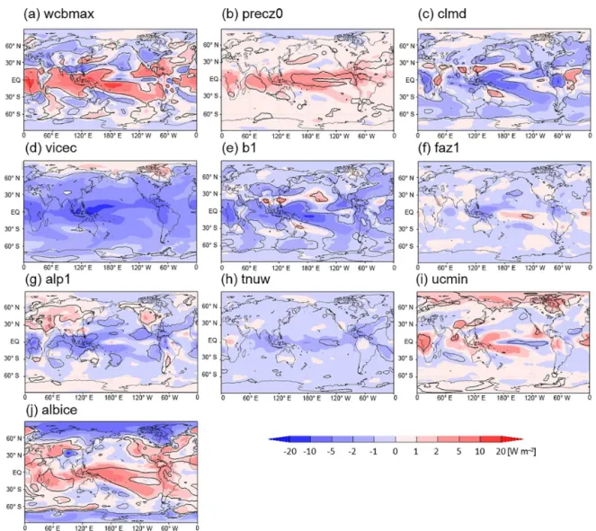
Focusing on the longwave CRE, we find that the most ef-fective parameters are wcbmax and vicec; wcbmax and vicec can change the LCRE by more than 10 W m−2
at low lati-tudes (Fig. 8a, d).
Increasing the wcbmax leads to changes in the cloud top pressure, which decreases in tropical Africa, western tropical Pacific, and the South Pacific Convergence Zone, while it in-creases in the subtropics, especially around South and South-east Asia (Fig. A3a). The decrease (increase) in the cloud top pressure would lead to a decrease (increase) in the cloud top temperature and upward longwave radiation, which would contribute to the increase (decrease) in the greenhouse effect of clouds and the LCRE. The geographical distribution of the changes in the cloud top pressure and LCRE are similar to each other, which is consistent with the above-mentioned argument (Figs. A3a, 8a).
Figure 8.Regression coefficient of the annual mean TOA longwave CRE on the tuning parameters calculated using the 56 samples of the MIROC5 PPE. The definition of the tuning parameters is shown in Table 1. The tuning parameters are normalized to the range of [0, 1]. The black curves indicate the threshold of the statistical significance with the 5 % level.
the greenhouse effect of clouds, which is consistent with the decrease in LCRE, as shown in Fig. 8d.
6 Discussion
The results of the present study have implications for the future development of MIROC. Parameter tuning has only a limited capability to control the SCRE biases over low-latitude oceans and the Southern Ocean in MIROC5. There-fore, modifying the model structure should be given a high priority to effectively alleviate the biases. The results under-line the importance of improving parameterizations based on cloud process studies. On the other hand, the SCRE bias in the Arctic can be fully controlled by tuning the albedo of snow and ice in the current model structure. However, we expect that the albedo will be predicted or diagnosed with a more physically based parameterization in the future rather
than being specified as a tuning parameter, which would make the tuning of the SCRE more difficult.
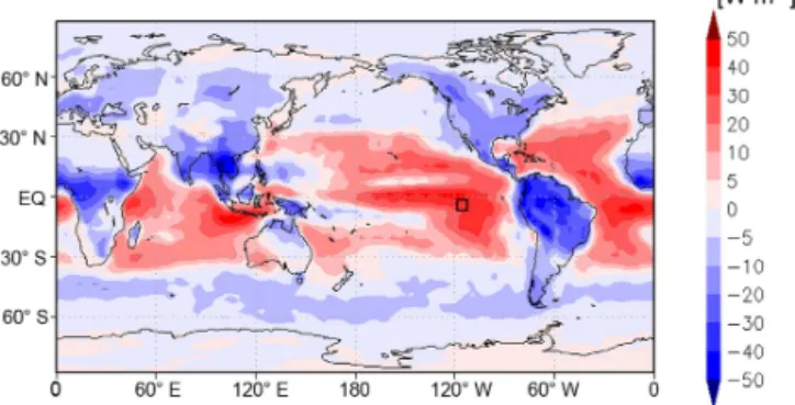
Figure 9.Changes in annual mean TOA shortwave CRE induced by implementing a shallow convection parameterization and parame-ter tuning in the MIROC5 AGCM. The black square in the easparame-tern tropical Pacific indicates the position of a grid point focused on in Fig. 10.
oceans, which alleviates the negative SCRE bias (Figs. 3a and 9).
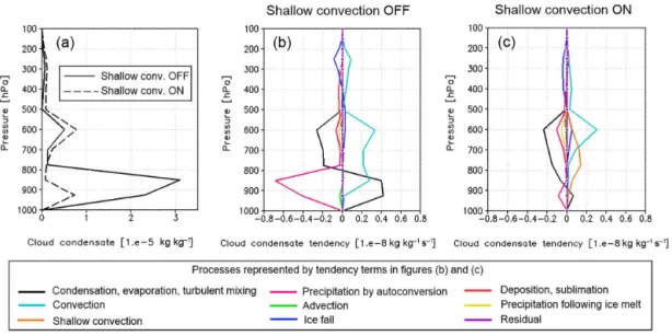
As an illustration, we focus on a grid point in the east-ern tropical Pacific and look at the vertical profile of cloud condensate (liquid plus ice) and its tendency in Fig. 10. We find a large maximum of cloud condensate at 850 hPa before the implementation of the shallow convection scheme (solid line in Fig. 10a). This maximum is maintained by increasing tendencies from condensation, evaporation, turbulent mix-ing, and convection (black and light blue lines in Fig. 10b), and also by decreasing tendency from precipitation (magenta line in Fig. 10b). After the implementation, those tendencies become smaller than before (Fig. 10c), and the maximum of cloud condensate at 850 hPa disappears (broken line in Fig. 10a). There appears an increasing tendency from shal-low convection at upper levels around 600–800 hPa (orange line in Fig. 10c), but this does not lead to large increase in cloud condensate. The obtained results are consistent with the view that vertical mixing induced by shallow convection causes upward transport of total water in the lower tropo-sphere, which dehydrates the low-cloud layer and decreases the low cloud condensate, thereby making the SCRE less negative.
As a next step, research concerning the impact of shallow convection on cloud feedback would also be useful. Previous studies indicate that simulated strength of convective mixing between the lower and middle tropical troposphere is related to cloud feedback and climate sensitivity in multi-model en-sembles (Sherwood et al., 2014; Kamae et al., 2016). The results suggest that shallow convective mixing contributes to inter-model spread in climate sensitivity, which causes diffi-culty in assessing the impact of climate change. In order to test the hypothesis, a multi-model comparison is proposed in which climate feedback is estimated with shallow convection turned on and off in AGCMs. The comparison is called Se-lected Process On/Off Klima Inter-comparison Experiment (SPOOKIE) phase 2, which is under the framework of Cloud
Feedback Model Inter-comparison Project (CFMIP, Webb et al., 2017). We expect that the SPOOKIE phase 2 will facili-tate better understanding of the connection between shallow convection and cloud feedback.
The present study also has implications for the inter-model difference in the CRE simulated by the CMIP5 MME. The SCRE and LCRE simulated by the CMIP5 MME show a large inter-model spread. The spread is larger than that in the MIROC5 PPE; therefore, the observation data are within the range of the CMIP5 ensemble members for both the global mean and the zonal mean values (Dolinar et al., 2015; Flato et al., 2013). This large spread in the CMIP5 MME stems from the inter-model difference in both the model structure and specified parameter settings. The results of the present study indicate that specified parameter settings can explain only a small part of the inter-model spread in the CMIP5 MME, suggesting that most of the spread is attributable to the difference in the model structure. This is consistent with the view that modifying the model structure is important for alleviating the biases in SCRE and LCRE.
However, we should note that the results of the model eval-uation presented here depend on the design of the PPE exper-iment. For example, we restricted the number of perturbed parameters to 10 and that of the PPE members to 56 based on the number of available computational resources. If we in-creased the number of perturbed parameters and PPE mem-bers, the inter-model difference of the TOA radiation and cloud biases might be larger than that of the present study. The importance of the PPE design in obtaining large inter-model spread is illustrated by Yamazaki et al. (2013), who conducted a PPE experiment with an AOGCM, HadCM3. They perturbed 33 parameters to create 20 000 members in the PPE experiment. Although they subsampled the PPE members so that the TOA radiation balance is close to the observation, as was done by Shiogama et al. (2012), they showed that the inter-model difference of the climate sen-sitivity is larger than that of the MIROC5 PPE or the CMIP MME.
The choice of the model used for the PPE experiment is another important factor. If we employed a model other than MIROC5, the biases in the TOA radiation and clouds would be notably different from what we presented. Klein et al. (2013) reported that the bias of having too many optically thick clouds has been reduced from CFMIP1 to CFMIP2 MME, with the best models having eliminated this bias. If we used a model with a very small bias in optically thick clouds, we might be able to change the sign of the bias by parameter tuning only. Therefore, the dominance of structure-oriented bias as illustrated by the MIROC5 PPE does not necessar-ily indicate unimportance of the parameter-oriented bias in general, as the latter is a function of the former.
Figure 10.Vertical profile of annual mean(a)cloud condensate and(b, c)cloud condensate tendencies in the eastern tropical Pacific simu-lated by the MIROC5 AGCM. The data are from the grid point located at (114◦
W, 5◦
S), indicated by the black square in Fig. 9.(a)Cloud condensate simulated without shallow convection parameterization (solid line) and with the parameterization (broken line),(b)cloud con-densate tendencies simulated without shallow convection parameterization, and(c)cloud condensate tendencies simulated with the parame-terization.
However, such models could also be included in the PPE if we applied flux adjustment at the sea surface to suppress cli-mate drift, which might increase the parametric uncertainty of the biases compared with the present study. For example, Yamazaki et al. (2013) reported that the parametric uncer-tainty of the climate sensitivity increases by adopting models with a large TOA radiation imbalance in their PPE experi-ment using the HadCM3 AOGCM. Collins et al. (2006) also conducted a PPE experiment using the HadCM3 AOGCM with flux adjustment. They showed that the parametric un-certainty of the TOA shortwave radiation in the global and annual mean is∼20 W m−2, which is much larger than the
results in the present study.
If we did not adopt the SIS method in the MIROC5 PPE, namely, if we included PPE members with large TOA radia-tion imbalance by applying flux adjustment, how much larger would the inter-model spread become compared with this study? To address this issue, we estimated inter-model spread of the TOA net radiation in the MIROC5 PPE for two sets of ensemble members: (1) 5000 members created with Latin hy-percube sampling, which include members with large TOA radiative imbalance, and (2) 56 members with small TOA ra-diative imbalance, which are selected with the SIS method from the 5000 members in (1). We estimated the standard deviation for the two sets of ensemble members, and the ra-tio of (1) to (2) is 6.25 to 1.0. Therefore, inter-model spread of the TOA net radiation would be about 6 times larger if we did not adopt the SIS method. For the sake of argument, we now assume that the 6-fold increase in the inter-model spread occurs not only to the net radiation, but also to the SCRE. In this case, observation data would be within the range of the
PPE spread in the global mean SCRE, in contrast to what we have seen in Fig. 1c. However, as for the SCRE over the sub-tropical oceans as seen in Fig. 3a, the observation data would still be outside the range of the PPE. The above arguments are consistent with Yokohata et al. (2012), who evaluated the SCRE bias of PPE experiments under present climate condi-tions. They used output of the PPEs conducted with multiple GCMs, some of which employed flux adjustment, and find that the SCRE cooling bias over the subtropical oceans ap-pears in almost all PPE members.
7 Conclusions
parameters such as the maximum cumulus updraft velocity at the cloud base. On the other hand, the bias of the SCRE in the Arctic was sensitive to parameter tuning. It could be removed by tuning parameters such as the albedo of ice and snow both in the zonal mean and at each grid point.
As discussed in Sect. 6, the obtained results of the PPE experiment are dependent on the model and experimental design. In particular, inter-model spread of the PPE is af-fected by employing the SIS method. Whether the results are applicable to other models or PPE experiments remains to be investigated further. However, the present study illus-trates the benefit of PPE experiments, which provide use-ful information regarding the model development strategy, namely, the effectiveness and limitations of parameter tun-ing. Based on the results of the present study, a parameteri-zation for shallow convection was implemented in MIROC6 to alleviate the cloud bias over low-latitude oceans. Conduct-ing PPE experiments with the future versions of MIROC is advisable to update our knowledge about the parametric un-certainty, which depends on the model structure; PPE exper-iments without flux adjustment using AOGCMs other than MIROC5 would also be useful for evaluating the biases in the simulated present climates, which are relevant for future projections in the CMIP5 MME.
Appendix A: Impact of parameter tuning on ISCCP cloud properties
The regression coefficients of the ISCCP cloud properties (cloud amount, cloud optical thickness, and cloud top pres-sure) on tuning parameters are shown here to help readers interpret the CRE changes in Figs. 7 and 8.
Competing interests. The authors declare that they have no conflict of interest.
Acknowledgements. The authors thank Hideaki Kawai and two anonymous reviewers for valuable discussion and comments. The authors also thank Editage (www.editage.jp) for English language editing. This work was supported by the Program for Risk Infor-mation on Climate Change and the Integrated Research Program for Advancing Climate Models of the Ministry of Education, Culture, Sports, Science and Technology (MEXT), Japan. HS was supported by Grant-in-Aid 26281013 from the MEXT of Japan. The Earth Simulator at JAMSTEC and NEC SX at NIES were used to perform the model simulations.
Edited by: Holger Tost
Reviewed by: two anonymous referees
References
Barkstrom, B. R.: The Earth Radiation Budget Experiment (ERBE), B. Am. Meteorol. Soc., 65, 1170–1185, 1984.
Bodas-Salcedo, A., Webb, M. J., Bony, S., Chepfer, H., Dufresne, J.-L., Klein, S. A., Zhang, Y., Marchand, R., Haynes, J. M., Pin-cus, R., and John, V. O.: COSP-satellite simulation software for model assessment, B. Am. Meteorol. Soc., 92, 1023–1043, 2011. Bodas-Salcedo, A., Williams, K. D., Ringer, M. A., Beau, I., Cole, J. N. S., Dufresne, J.-L., Koshiro, T., Stevens, B., Wang, Z., and Yokohata, T.: Origins of the solar radiation biases over the South-ern Ocean in CFMIP2 models, J. Climate, 27, 41–56, 2014. Ceppi, P., Hwang, Y.-T., Frierson, D. M. W., and Hartmann, D. L.:
Southern Hemisphere jet latitude biases in CMIP5 models linked to shortwave cloud forcing, Geophys. Res. Lett., 39, L19708, https://doi.org/10.1029/2012GL053115, 2012.
Chepfer, H., Bony, S., Winker, D., Chiriaco, M., Dufresne, J.-L., and Seze, G.: Use of CALIPSO lidar observations to evaluate the cloudiness simulated by a climate model, Geophys. Res. Lett., 35, L15704, https://doi.org/10.1029/2008GL034207, 2008. Chepfer, H., Bony, S., Winker, D., Cesana, G., Dufresne, J.-L.,
Min-nis, P., Stubenrauch, C. J., and Zeng, S.: The GCM-oriented CALIPSO cloud product (CALIPSO-GOCCP), J. Geophys. Res., 115, D00H16, https://doi.org/10.1029/2009JD012251, 2010.
Chikira, M. and Sugiyama, M.: A cumulus parameterization with state-dependent entrainment rate. Part 1: description and sensi-tivity to temperature and humidity profiles, J. Atmos. Sci., 67, 2171–2193, 2010.
Collins, M., Booth, B. B. B., Harris, G. R., Murphy, J. M., Sexton, D. M. H., and Webb, M. J.: Towards quantifying uncertainty in transient climate change, Clim. Dynam., 27, 127–147, 2006. Dolinar, E. K., Dong, X., Xi, B., Jiang, J. H., and Su, H.:
Evalua-tion of CMIP5 simulated clouds and TOA radiaEvalua-tion budgets us-ing NASA satellite observations, Clim. Dynam., 44, 2229–2247, https://doi.org/10.1007/s00382-014-2158-9, 2015.
Flato, G., Marotzke, J., Abiodun, B., Braconnot, P., Chou, S. C., Collins, W., Cox, P., Driouech, F., Emori, S., Eyring, V., Forest, C., Gleckler, P., Guilyardi, E., Jakob, C., Kattsov, V., Reason, C., and Rummukainen, M.: Evaluation of Climate Models. in:
Cli-mate Change 2013: The Physical Science Basis. Contribution of Working Group 1 to the Fifth Assessment Report of the Inter-governmental Panel on Climate Change, edited by: Stocker, T. F., Qin, D., Plattner, G.-K., Tignor, M., Allen, S. K., Boschung, J., Nauels, A., Xia, Y., Bex, V., and Midgley, P. M., Cambridge University Press, Cambridge, United Kingdom and New York, NY, USA, 2013.
Jackson, L. C., Vellinga, M., and Harris, G. R.: The sensitivity of the meridional overturning circulation to modelling uncertainty in a perturbed physics ensemble without flux adjustment, Clim. Dynam., 39, 277–285, 2012.
Kamae, Y., Shiogama, H., Watanabe, M., Ogura, T., Yokohata, T., and Kimoto, M.: Lower-tropospheric mixing as a constraint on cloud feedback in a multiparameter multiphysics ensemble, J. Climate, 29, 6259–6275, 2016.
Klein, S. A. and Jakob, C.: Validation and sensitivities of frontal clouds simulated by the ECMWF model, Mon. Weather Rev., 127, 2514–2531, 1999.
Klein, S. A., Zhang, Y., Zelinka, M. D., Pincus, R., Boyle, J., and Gleckler, P. J.: Are climate model simulations of clouds improv-ing? An evaluation using the ISCCP simulator, J. Geophys. Res., 118, 1329–1342, 2013.
Loeb, N. G., Wielicki, B. A., Doelling, D. R., Smith, G. L., Keyes, D. F., Kato, S., Manalo-Smith, N., and Wong, T.: Toward opti-mal closure of the Earth’s top-of-atmosphere radiation budget, J. Climate, 22, 748–766, 2009.
Murphy, J. M., Sexton, D. M. H., Barnett, D. N., Jones, G. S., Webb, M. J., Collins, M., and Stainforth, D. A.: Quantification of mod-elling uncertainties in a large ensemble of climate change simu-lations, Nature, 430, 768–772, 2004.
Nakanishi, M. and Niino, H.: An improved Mellor-Yamada level-3 model with condensation physics: its design and verification, Bound.-Lay. Meteorol., 112, 1–31, 2004.
Nam, C., Bony, S., Dufresne, J.-L., and Chepfer, H.: The ‘too few, too bright’ tropical low-cloud problem in CMIP5 models, Geophys. Res. Lett., 39, L21801, https://doi.org/10.1029/2012GL053421, 2012.
Park, S. and Bretherton, C. S.: The University of Washington shal-low convection and moist turbulence schemes and their impact on climate simulations with the Community Atmosphere Model, J. Climate, 22, 3449–3469, 2009.
Pincus, R., Platnick, S., Ackerman, S. A., Hemler, R. S., and Hof-mann, R. J. P.: Reconciling simulated and observed views of clouds: MODIS, ISCCP, and the limits of instrument simulators, J. Climate 25, 4699–4720, 2012.
Rossow, W. B., Walker, A. W., Beuschel, D., and Roiter, M.: In-ternational Satellite Cloud Climatology Project (ISCCP) docu-mentation of new cloud datasets, World Climate Research Pro-gramme (ICSU and WMO), WMO/TD 737, 115 pp., 1996. Sherwood, S. C., Bony, S., and Dufresne, J.-L.: Spread in model
climate sensitivity traced to atmospheric convective mixing, Na-ture, 505, 37–42, 2014.
Takata, K., Emori, S., and Watanabe, T.: Development of the minimal advanced treatments of surface interaction and runoff, Global Planet. Change, 38, 209–222, 2003.
Takemura, T., Nozawa, T., Emori, S., Nakajima, T. Y., and Naka-jima, T.: Simulation of climate response to aerosol direct and in-direct effects with aerosol transport-radiation model, J. Geophys. Res., 110, D02202, https://doi.org/10.1029/2004JD005029, 2005.
Takemura, T., Egashira, M., Matsuzawa, K., Ichijo, H., O’ishi, R., and Abe-Ouchi, A.: A simulation of the global dis-tribution and radiative forcing of soil dust aerosols at the Last Glacial Maximum, Atmos. Chem. Phys., 9, 3061–3073, https://doi.org/10.5194/acp-9-3061-2009, 2009.
Trenberth, K. E. and Fasullo, J. T.: Simulation of present-day and twenty-first-century energy budgets of the southern oceans, J. Climate, 23, 440–454, 2010.
Watanabe, M., Emori, S., Satoh, M., and Miura, H.: A PDF-based hybrid prognostic cloud scheme for general circulation models, Clim. Dynam., 33, 795–816, 2009.
Watanabe, M., Suzuki, T., O’ishi, R., Komuro, Y., Watanabe, S., Emori, S., Takemura, T., Chikira, M., Ogura, T., Sekiguchi, M., Takata, K., Yamazaki, D., Yokohata, T., Nozawa, T., Hasumi, H., Tatebe, H., and Kimoto, M.: Improved climate simulation by MIROC5: mean states, variability, and climate sensitivity, J. Cli-mate, 23, 6312–6335, 2010.
Webb, M., Senior, C., Bony, S., and Morcrette, J. J.: Combining ERBE and ISCCP data to assess clouds in the Hadley Centre, ECMWF and LMD atmospheric climate models, Clim. Dynam., 17, 905–922, 2001.
Webb, M. J., Andrews, T., Bodas-Salcedo, A., Bony, S., Brether-ton, C. S., Chadwick, R., Chepfer, H., Douville, H., Good, P., Kay, J. E., Klein, S. A., Marchand, R., Medeiros, B., Siebesma, A. P., Skinner, C. B., Stevens, B., Tselioudis, G., Tsushima, Y., and Watanabe, M.: The Cloud Feedback Model Intercomparison Project (CFMIP) contribution to CMIP6, Geosci. Model Dev., 10, 359–384, https://doi.org/10.5194/gmd-10-359-2017, 2017. Wielicki, B. A., Barkstrom, B. R., Harrison, E. F., Lee III, R. B.,
Smith, G. L., and Cooper, J. E.: Clouds and the Earth’s Radi-ant Energy System (CERES): An Earth observing system exper-iment, B. Am. Meteorol. Soc., 77, 853–868, 1996.
Wilson, D. R. and Ballard, S. P.: A microphysically based precipi-tation scheme for the UK Meteorological Office Unified Model, Q. J. Roy. Meteor. Soc., 125, 1607–1636, 1999.
Yamazaki, K., Rowlands, D. J., Aina, T., Blaker, A. T., Bowery, A., Massey, N., Miller, J., Rye, C., Tett, S. F. B., Williamson, D., Ya-mazaki, Y. H., and Allen, M. R.: Obtaining diverse behaviors in a climate model without the use of flux adjustments, J. Geophys. Res., 118, 2781–2793, 2013.
Yokohata, T., Annan, J. D., Collins, M., Jackson, C. S., Tobis, M., Webb, M. J., and Hargreaves, J. C.: Reliability of multi-model and structurally different single-multi-model ensembles, Clim. Dynam., 39, 599–616, 2012.
Zelinka, M. D., Klein, S. A., and Hartmann, D. L.: Computing and partitioning cloud feedbacks using cloud property histograms. Part 1: Cloud radiative kernels, J. Climate, 25, 3715–3735, 2012. Zhang, M. H., Lin, W. Y., Klein, S. A., Bacmeister, J. T., Bony, S., Cederwall, R. T., Del Genio, A. D., Hack, J. J., Loeb, N. G., Lohmann, U., Minnis, P., Musat, I., Pincus, R., Stier, P., Suarez, M. J., Webb, M. J., Wu, J. B., Xie, S. C., Yao, M.-S., and Zhang, J. H.: Comparing clouds and their sea-sonal variations in 10 atmospheric general circulation models with satellite measurements, J. Geophys. Res., 110, D15S02, https://doi.org/10.1029/2004JD005021, 2005.
Zhang, Y., Rossow, W. B., Lacis, A. A., Oinas, V., and Mishchenko, M. I.: Calculation of radiative fluxes from the surface to top of atmosphere based on ISCCP and other global data sets: Refinements of the radiative transfer model and the input data, J. Geophys. Res., 109, D19105, https://doi.org/10.1029/2003JD004457, 2004.