169
Deposit Competition and Financial Fragility: Evidence from
the US Banking Sector
†By Mark Egan, Ali Hortaçsu, and Gregor Matvos*
We develop a structural empirical model of the US banking sector. Insured depositors and run-prone uninsured depositors choose between differentiated banks. Banks compete for deposits and endogenously default. The estimated demand for uninsured deposits
declines with banks’ inancial distress, which is not the case for
insured deposits. We calibrate the supply side of the model. The calibrated model possesses multiple equilibria with bank-run
features, suggesting that banks can be very fragile. We use our model
to analyze proposed bank regulations. For example, our results
suggest that a capital requirement below 18 percent can lead to
signiicant instability in the banking system. (JEL E44, G01, G21,
G28, G32)
The recent inancial crisis has brought renewed attention to the stability of the banking sector. An extensive theoretical literature allows us to understand the mech-anisms underlying banking (in)stability (Diamond and Dybvig 1983, Goldstein and Pauzner 2005).1 These models have also provided a rich environment to study the
qualitative consequences of policy interventions. These qualitative models, how-ever, were not designed to address quantitative questions. For example, Diamond-Dybvig (1983) style models imply that equilibria in which banks are unstable might exist, but do not tell us how bad these equilibria would be given the fundamentals of the US banking sector. We ill this gap by developing a quantitative model of the
1 See also, Postlewaite and Vives (1987); Cooper and Ross (1998); Peck and Shell (2003); Allen and Gale
(2004); Rochet and Vives (2004); Farhi, Golosov, and Tsyvinski (2009); Gertler and Kiyotaki (2015); and Kashyap, Tsomocos, and Vardoulakis (2014).
* Egan: Carlson School of Management, University of Minnesota, 321 19th Avenue S., Minneapolis, MN 55455 (e-mail: [email protected]); Hortaçsu: Department of Economics, University of Chicago, 1126 E. 59th Street, Chicago, IL 60637 (e-mail: [email protected]); Matvos: Booth School of Business, University of Chicago, 5807 S. Woodlawn Avenue, Chicago, IL 60637 (e-mail: [email protected]).We thank Jose Ignacio Cuesta for outstanding research assistance. We are also grateful for comments and helpful suggestions by Victor Aguirregabiria, Robert Clark, Dean Corbae, Douglas Diamond, Lars Hansen, Ginger Jin, Anil Kashyap, Rafael Repullo, John Rust, Marc Rysman, David Scharfstein, Rob Vishny, and the seminar participants at Chicago Booth Microeconomics Lunch, Chicago Booth Finance Workshop, Chicago Money and Banking Seminar, Duke University, Harvard University, the Minneapolis Federal Reserve, New York University, University of Tokyo, University of Utah, University of Calgary Empirical Microeconomics Workshop, the Society for Economic Dynamics Meetings, the Financial Intermediation Research Society Conference, Wharton Conference on Liquidity and Financial Crises, Econometric Society North American Meetings, and the NBER Industrial Organization Program Meeting. Ali Hortaçsu acknowledges inancial support of the NSF (SES 1426823). The authors declare that they have no relevant or material inancial interests that relate to the research described in this paper. All errors are our own.
US banking sector. As in Diamond and Dybvig (1983) and Goldstein and Pauzner (2005), uninsured depositors are run prone and are the main source of instability in the banking sector. Differentiated banks compete for uninsured and insured depos-itors, and endogenously default. We estimate and calibrate the model on a new dataset covering the largest US banks over the period 2002–2013. We ind that the uninsured deposit elasticity to bank default is large enough to introduce the possibil-ity of alternative equilibria in which banks are substantially more likely to default. We study how competition for deposits among banks affects the feedback between bank distress and deposits, and transmits shocks from one bank to the system. Last, we use our model to analyze the proposed bank regulatory changes and ind that some regulations could exacerbate the instability of the system. Our results sug-gest that capital requirements below 18 percent allow for equilibria with substantial probabilities of bank default and large welfare losses.2
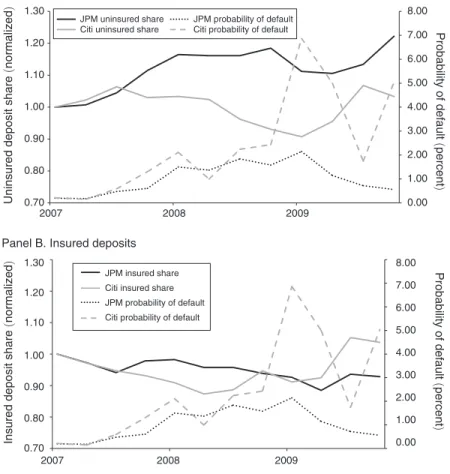
Deposits represent over three-quarters of funding of US commercial banks (Hanson et al. 2015). Moreover, in the largest commercial banks, approximately half of deposits are uninsured. Uninsured deposits are frequently impaired in cases of bank default,3 and are therefore potentially prone to runs. Figure 1 suggests that
inancial distress of banks affects their ability to attract uninsured deposits. We plot the relationship between the uninsured deposit market shares and inancial distress for Citibank and JPMorgan Chase from 2005 through 2010. As distress4 of Citibank
increases relative to JPMorgan, Citi’s market share of uninsured deposits decreases and JPMorgan’s market share increases (panel A). Note that the market shares of insured deposits, which should be insensitive to distress, show no such relation-ship (panel B). The existing literature suggests that uninsured deposits can lead to bank instability and be subject to self-reinforcing runs (Diamond and Dybvig 1983, Goldstein and Pauzner 2005). Such feedback mechanisms can even result in multi-ple equilibria.
Whether such feedback mechanisms can lead to multiple equilibria depends on the sensitivity of uninsured depositors to bank distress, on which there is little systematic evidence. In principle, uninsured depositors should be very sensitive to potential bank default. In Diamond and Dybvig (1983), as soon as depositors think their deposits could be impaired, they withdraw, thereby triggering bank default. Alternatively, the Basel Committee on Banking Supervision (2013) considers unin-sured deposits as the second most stable source of funding after inunin-sured depositors. If uninsured deposits are not very responsive to bank distress, because this bank provides payroll services or manages receivables for the depositor, then the danger of a panic run would be diminished. Even if the estimates were available, the liter-ature provides little guidance on whether the elasticity is large enough to result in self-reinforcing runs or multiple equilibria.5 The strength of the feedback between
deposits and inancial distress also depends on how costly deposit withdrawals are
2 The Financial Stability Board, a group of international regulators, has proposed total loss-absorbing capacity of large banks, which is the equivalent of our capital requirements, of 16–20 percent of assets.
3 The FDIC reports that only approximately 25 percent of transactions transfer all deposits, including the unin-sured, to a new institution. https://www.fdic.gov/bank/individual/failed/wamu_q_and_a.html (accessed December 28,2014).
4 We measure distress using credit default swap spreads (CDS).
for a bank, and how a bank responds to a raised probability of withdrawals (for example, by raising interest rates). To quantify these forces, we develop a model of retail banking, which we calibrate using data for large US banks.
Demand for deposits in our model is driven by several forces. First, as is stan-dard in bank run models, the demand for uninsured deposits depends on the inan-cial health of the bank, because these deposits may be impaired in case of bank default. Casual observation suggests that US commercial banks are differentiated. For example, Citi offers a somewhat larger ATM network than Fifth Third Bank and has had substantially fewer complaints against it iled by customers at the Consumer Financial Protection Bureau on a per customer basis. Large and persistent differ-ences in banks’ market shares suggest that product differentiation plays an important role in US commercial banking. We therefore depart from the current literature by adding product differentiation between banks. The properties of the demand func-tion, especially the elasticity of uninsured deposit demand with respect to inancial distress, provide substantial discipline on the magnitude of self-fulilling runs that the model can generate.
The second force, which determines the strength of the feedback, is the behav-ior of banks. Banks compete for insured and uninsured deposits by setting interest
0.00 1.00 2.00 3.00 4.00 5.00 6.00 7.00 8.00 0.70 0.80 0.90 1.00 1.10 1.20 1.30
2007 2008 2009
Probability of default
(
percent
)
Uninsured deposit share
(
normalized
)
Panel A. Uninsured deposits
JPM uninsured share Citi uninsured share
JPM probability of default Citi probability of default
0.00 1.00 2.00 3.00 4.00 5.00 6.00 7.00 8.00 0.70 0.80 0.90 1.00 1.10 1.20 1.30
2007 2008 2009
Probability of default
(
percent
)
Insured deposit share
(
normalized
)
Panel B. Insured deposits
JPM insured share Citi insured share
JPM probability of default
Citi probability of default
rates in a standard Bertrand-Nash differentiated products setting (Matutes and Vives 1996). Banks earn stochastic returns on deposits net of other operational costs. We model banks’ endogenous default decisions in a simple framework based on Leland (1994). Each period, equity holders decide whether to continue operations by repay-ing deposits and the long-term debt coupon. Alternatively, banks can declare bank-ruptcy, which is anticipated by rational depositors. Because consumers are sensitive to inancial distress, a bank in inancial distress has to offer higher interest rates on its deposits, which decreases its proitability. We take this model to the data by irst estimating demand for deposits and then calibrating the supply side of the model.
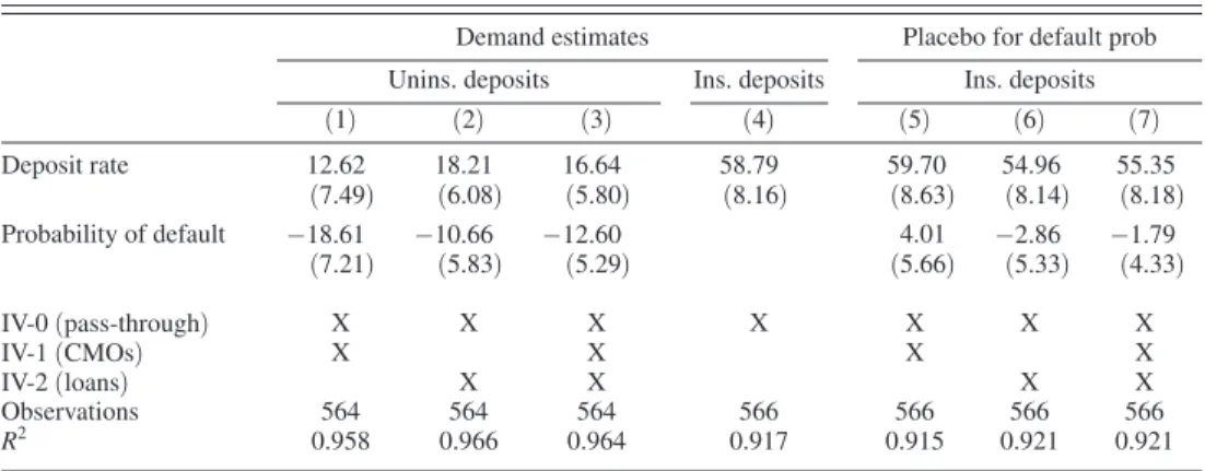
We estimate demand using variation in banks’ inancial distress, interest rates on deposits, and bank market shares using a standard model of demand (Berry 1994; Berry, Levinsohn, and Pakes 1995 (BLP)). To illustrate the effect of inancial dis-tress on demand for uninsured deposits, we irst estimate a triple-difference speci-ication with bank and time ixed effects. We ind that as a bank’s inancial distress increases, the market share of its uninsured deposits declines relative to its share of insured deposits, suggesting that demand for uninsured deposits declines with a bank’s inancial distress. We provide complementary evidence exploiting varia-tion in banks’ inancial distress resulting from changes in banks’ portfolio holdings and performance, and ind similar results. Contrary to uninsured deposits, we ind no evidence that insured deposits are sensitive to banks’ inancial distress. Jointly, several sources of variation paint the same picture that uninsured depositors are run prone: as a bank’s default probability increases, the demand for uninsured deposits decreases. The effect is substantial: a 100 basis point increase in the risk-neutral probability of bankruptcy results in a 12 percent market share decline.
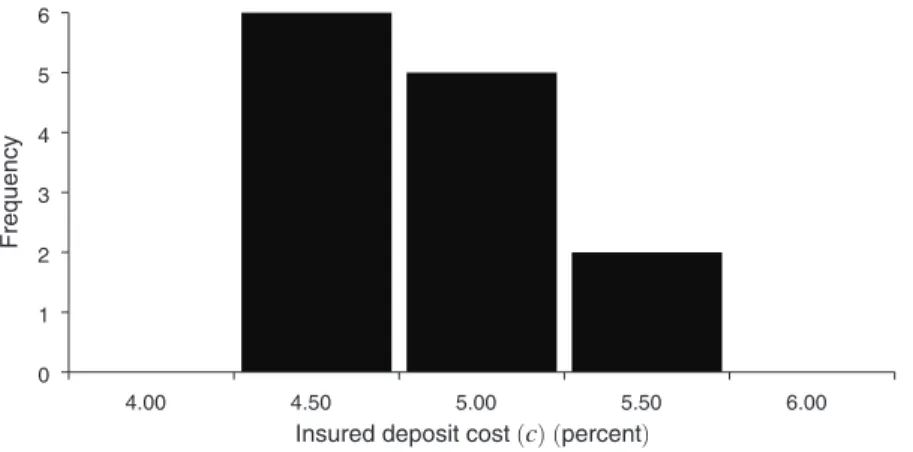
To obtain supply-side parameters, which govern banks’ behavior, we calibrate the model using revealed preferences of banks. Banks optimally set interest rates on insured and uninsured deposits, and choose when to default. With the addition of demand estimates, banks’ optimality conditions allow us to calibrate the quantities we do not observe, the mean and variance of returns on deposits for each bank, as well as the additional noninterest costs of servicing insured deposits that recon-cile the behavior of banks with observed quantities. We solve for the parameters in closed form and show that the parameters are exactly and uniquely identiied. For any observed equilibrium of the game, there is a unique set of parameters that rationalizes the data. Even though the baseline model is fairly simple and sparse, the calibration yields reasonable results on quantities, which were not used to calibrate the model. For example, the implied bank proitability is approximately 2.9 percent to 3.75 percent, which is similar to balance sheet measures of proitability in Hanson et al. (2015) and Hirtle et al. (2014) of 2 percent to 2.5 percent.
would correctly believe that Wachovia was more likely to default and would with-draw their deposits, which would in turn lower the proitability of Wachovia and increase its probability of default. Our estimates suggest that if the equilibrium changes, then seemingly stable banks can quickly become unstable with no change in their fundamentals.
Several broad facts emerge from our analysis of multiple equilibria. First, the banking system was in the best equilibrium for much of the period we study and close to the best in the rest of it. Second, substantially worse equilibria with large welfare losses, in which each bank has a higher default probability and some banks are highly unstable, also exist. This instability of one bank can spill over to other banks even without direct linkages between banks. A bank with a high probability of default is willing to offer high insured deposit rates, because FDIC insurance bears their cost with a high probability. To compete for these deposits, other banks increase rates as well, which decreases their margins and increases their distress. This argument was used by the FDIC when it successfully pressured Ally Bank to lower its deposit rates in 2009 (Leiber 2009).
Last, in all equilibria, several banks remain active, and provide depositor services to a large part of the market. Depositors value banking services, and as more banks are distressed, the demand for deposits shifts to relatively healthier banks. These results suggest that a mechanism that could destabilize the whole banking system would have to involve direct linkages across banks, which would overcome the force for stability we describe above.
Overall, we provide a workhorse model that allows us to evaluate the stability of the banking system in the presence of run-prone uninsured deposits. We use the model to show that the large amounts of uninsured deposits in the US commercial banking system can lead to severely unstable banks, given the elasticity of uninsured deposits to inancial distress. We then use our calibrated model to assess some recent and proposed bank regulatory changes. We analyze the effect of interest rate caps on insured deposits,6 and ind that they limit the worst possible losses to the FDIC.
We also ind that increasing FDIC insurance mostly transfers rents to newly insured depositors without large improvements to banking stability, but that the results of this seemingly simple policy critically depend on the preferences of newly insured depositors. Conversely, we ind evidence suggesting that imposing bank risk limits may be counterproductive and could actually decrease stability in the banking sector.
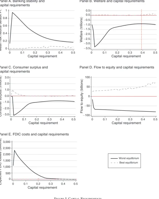
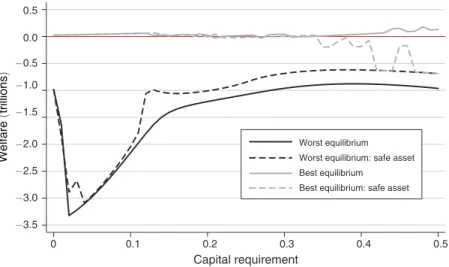
We use our model to quantitatively study the effect of capital requirements. Increasing capital requirements decreases the severity of the largest possible insta-bility in the banking sector, but also eliminates some equilibria in which the banking system is very stable. We ind that banking stability and welfare do not necessarily go hand in hand. Increasing capital requirements past a certain point decreases wel-fare even if it increases banking stability. Last, we show that capital requirements above 18 percent eliminate the possibility of equilibria with large welfare losses.
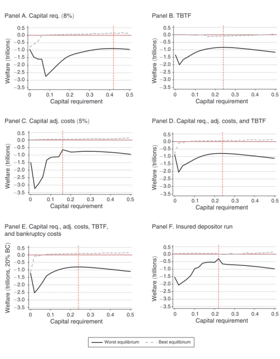
To allow for a rich and more realistic analysis of policy, we explore several extensions of the model. Because our analysis focuses on large US banks, we allow the government to save banks from bankruptcy through recapitalization, capturing
some features of too-big-to-fail policies. We also incorporate costly equity issuance and bankruptcy costs. These extensions have little impact on parameter estimates. Perhaps more surprisingly, while these extensions signiicantly alter the welfare cost of default, the basic consequences of capital requirements remain largely unchanged. Similar to the baseline model, capital requirements above 18 percent eliminate the possibility of equilibria with large welfare losses. Under a max–min welfare cri-terion,7 these capital requirements are optimal, exceed the 8 percent requirements
proposed under Basel III accords, and are quite close to the 16–20 percent total loss-absorbing capacity proposed by the Financial Stability Board.
Our policy conclusions are clearly limited to the speciic setting we examine. One can consider situations in which depositors, even if they are insured, are sensitive to default. For example, if there are delays in accessing payouts from deposit insur-ance, such as in India, then insured depositors suffer in bank default even if they eventually recover their deposits (Iyer and Puri 2012). Alternatively, if depositors believe that the banking system is likely subject to capital controls or haircuts if banks are close to defaulting, as has been recently the case in Greece and Cyprus, they may want to withdraw insured deposits prior to bankruptcy as well.
Our empirical and theoretical analysis relates to several strands in the banking and industrial organization literature. Our banking model builds on the automaker model from Hortaçsu et al. (2011). Our model is also in the spirit of the existing literature on bank runs, inancial stability, and inancial regulation, including the seminal work of Diamond and Dybvig (1983), and more recently Postlewaite and Vives (1987); Cooper and Ross (1998); Peck and Shell (2003); Allen and Gale (2004); Rochet and Vives (2004); Goldstein and Pauzner (2005); Farhi, Golosov, and Tsyvinski (2009); Gertler and Kiyotaki (2015); and Kashyap, Tsomocos, and Vardoulakis (2014).8 Similar to Matutes and Vives (1996), our model emphasizes
the strategic interaction among banks through competition.9
Our paper follows the precedent of recent papers that estimate structural models of imperfect competition in the banking sector. Our BLP-style demand model is closely related to the work of Dick (2008), who estimates demand for deposits using FDIC data. Unfortunately, the FDIC branch-level data does not break deposits down by insured versus uninsured categories, hence we cannot utilize this level of disag-gregation in our estimation exercise. Our supply-side model focuses on the deposit rate-setting and (endogenous) bankruptcy decisions of banks. Aguirregabiria, Clark, and Wang (2013) estimate a model in which the branch networks of banks are deter-mined endogenously, and use their model to estimate banks’ revealed preference for geographical risk diversiication. Corbae and D’Erasmo (2013, 2014) provide dynamic equilibrium models of the banking sector with imperfect competition, and use their models to evaluate the counterfactual effects of banking regulations, such as capital requirements. Our model and empirical analysis focuses on (imperfect)
7 An uncertainty averse planner would choose such a criterion (Gilboa and Schmeidler 1989).
8 For purely information based models of bank runs, see Chari and Jagannathan (1988); Jacklin and Bhattacharya
(1988); Allen and Gale (1998); and Uhlig (2010).
competition in the market for deposits, with special attention to insured versus unin-sured deposits, and pays particular attention to the presence of multiple equilibria and the possibility of bank runs or run-type equilibria.
The empirical results of our paper correspond to the existing literature on empirical bank runs and deposit insurance (for an overview, see Goldstein 2013). Iyer and Puri (2012) use unique event study data to examine how depositors responded to inan-cial distress and a subsequent bank run for a large Indian bank. Kelly and Ó Gráda (2000) and Ó Gráda and White (2003) examine depositor runs using depositor-level data in a New York bank during nineteenth century banking panics. Our paper also relates to Gorton (1988), who examines the relationship between economic fun-damentals and banking crises between 1863 and 1914, and Calomiris and Mason (2003), who study the role bank fundamentals played in bank runs occurring during the Great Depression. The empirical indings from our demand estimates closely relate to the indings from Schumacher (2000) and Martinez Peria and Schmukler (2001), who examine how depositors respond to bank inancial distress during the banking crises that occurred in Argentina, Chile, and Mexico during the 1980s and 1990s. Lastly, our empirical results relate to Hortaçsu et al. (2013), who measure the cost of inancial distress in the automaker industry.
Our paper is also broadly linked to the literature which studies runs in other inancial markets, such as money market funds and the asset-backed commercial paper market (Jank and Wedow 2010; Acharya, Schnabl, and Suarez 2013; Covitz, Liang, and Suarez 2013; Kacperczyk and Schnabl 2013; Strahan and Tanyeri 2015; Schroth, Suarez, and Taylor 2014; and Schmidt, Timmermann, and Wermers 2016). The run-prone behavior of uninsured depositors is similar to strategic complemen-tarities in withdrawal behavior of mutual fund investors in Chen, Goldstein, and Jiang (2010).
The remainder of the paper is laid out as follows. Section I develops our theoret-ical model of the banking sector. Section II describes the data used to estimate the deposit demand system and calibrate our theoretical model. Section III estimates the demand system for both insured and uninsured deposits. Section IV calibrates the banking side of the model. Section V studies the structure of multiple equilib-ria in the banking sector. Section VI assesses the stability of the banking sector and evaluates several proposed bank regulations. Section VII, extends the model to incorporate several other features of the banking sector, including “too big to fail,” bankruptcy costs, costly external inance, and run-prone insured depositors. Last, Section VIII concludes the paper.
I. Model
want to fund the shortfall in the spirit of Leland (1994), or let the bank default. An alternative institutional interpretation of default in the model is that equity hold-ers are allowed to recapitalize the bank at the end of each period. Regulators then inspect whether the bank can repay all deposits and the debt that has come due. If not, the bank is taken into receivership. For example, investors led by the Texas Paciic Group, a private equity irm, injected $7 billion into Washington Mutual after regulators warned that it was inadequately capitalized. They chose not to recapital-ize again ive months later, allowing the bank to be taken into FDIC receivership.10
The basic model contains three features we require to quantitatively approach the US banking sector: run-prone depositors, bank differentiation, and endogenous default. On the other hand, we try to keep the model stripped down enough to con-vey the intuition behind the forces driving the model, and its estimation. We incor-porate additional features of banking and default in Section VII to allow for a richer and more realistic analysis of policy.
We proceed by irst setting up the model, describing depositors’ preferences, banks’ technology, and funding. We then solve for deposit demand within a period, given interest rates set by banks and banks’ expected default rates. Last, we char-acterize the equilibrium deposit rates and default decisions of a bank, given deposi-tors’ rational expectations of default decisions.
A. Model Framework
The model is in discrete time. Every period, a mass of M I consumers are
choos-ing among K banks to deposit insured deposits, and a mass of M N consumers are
choosing among the same banks to deposit uninsured deposits, taking interest rates and the probabilities of default as given. Banks are indexed by k and compete for
insured and uninsured deposits from consumers indexed by j . Within the period, the
timing is as follows:
• Banks set interest rates for insured and uninsured deposits i k,I t and ik, Nt ;
• Consumers choose where to deposit funds;
• Banks invest deposits, and banks’ proit shock is realized;
• Banks choose whether to repay deposits and the coupon on long-term debt, or
default.
The model is speciied under the risk neutral measure.11
Depositor preferences.—Demand for deposits at bank k at time t depends on the
interest rate the bank offers, the services it provides the depositor, and, for uninsured depositors, the probability that the bank will default. The uninsured depositor is
10 The Washington Mutual case is not an exception. While there is limited data on equity issuance of private banks, SNL Financial data reports at least 40 failed banks had obtained equity injections in the 2 years prior to failure, and 124 distinct banks that had later failed had 689 capital offerings from 2008 to 2015.
promised an interest rate i k,Nt , from which she derives utility α N i k,N t , in which α N
mea-sures depositors’ sensitivity to interest rates. In the event of a bankruptcy, uninsured depositors lose utility low γ > 0 with a risk-neutral probability ρ k,t , suffering an
expected utility loss of ρ k,t γ .
Depositors also derive utility from banking services: δ kN + ε j,Nk, t . Bank-speciic
ixed effects, δ kN , relect bank quality differences: all else equal, some banks offer
better services than others. In addition, depositors’ preferences for banks also dif-fer; some consumers prefer Bank of America, and others Wells Fargo, for example, because of the proximity of ATMs to their home. These differences are captured in the i.i.d. utility shock ε j,Nk, t . The total indirect utility derived by an uninsured
depos-itor j from bank k at time t is then as follows:
(1) u j,Nk, = α t N i k,N − ρ t k,t γ + δ kN + ε j,Nk, t .
The preferences of insured and uninsured depositors might differ. The indirect util-ity of insured depositors closely mirrors that of uninsured depositors, but insured depositors do not lose utility in case of bankruptcy, obtain potentially different bank-ing services, and differ in interest rate sensitivity (indexed by I ):
(2) u j,I = α k,t I i k,I + δ t kI + ε j,I . k,t
In Section VIIE we relax this assumption, and allow insured depositors to be sensitive to bankruptcy as well. This modiication will address the situation in which insured depositors succumb to panics, or they correctly believe that their deposits will be impaired with bankruptcy because deposit insurance will be violated, or capital controls will be imposed on the banking system.
Banks.—Banks compete for depositors, each seeking to maximize equity value.
A bank’s proit maximization problem involves a three-part decision process: setting its insured deposit rate, setting its uninsured deposit rate, and ultimately deciding to continue its operations or declare bankruptcy.
Banks earn proits by lending out deposits. Bank k earns a period t return on
deposits net of other (noninterest) costs R k,t . These returns already account for all
noninterest costs, such as costs of loan defaults, the costs of screening loans, pro-viding services to depositors, etc. These returns are stochastic,12 distributed under
the risk-neutral measure asRk, t ∼ N
(
μ k , σ k)
, and are i.i.d. across time, but can bearbitrarily correlated among banks.13 Note that these per-period returns can be
neg-ative if the bank invests in bad projects. Because we index the process with k , some
banks are, on average, better at using deposits than others, and these differences
12 We think about the risky asset as a composite of all risky and riskless assets a bank can invest in. While the bank cannot choose the risk of its portfolio in our model, we investigate the consequences of forcing the bank to invest its capital requirements into a riskless asset in Section VIID. We ind that the risk composition of the asset portfolio has nontrivial consequences regarding the effects of regulatory requirements on the stability of the banking sector.
are persistent. Differences arise because some banks invest these deposits better or because they have lower costs of servicing loans and deposits.
Servicing insured depositors can be more expensive than the uninsured deposi-tors, because of FDIC deposit insurance premiums and other additional costs banks incur with insured, typically smaller accounts. Banks therefore incur an additional cost of servicing insured depositors, c k , relative to uninsured depositors. A bank
whose market share of insured deposits is s k,I t and whose market share of
unin-sured deposits is s k,N t earns a gross return on deposits of M I s k,I t
(
1 + R k,t − c k)
+ M N sk,Nt
(
1 + Rk, t)
.Banks’ proits are reduced by interest payments on deposits. They have to repay deposits, including the interest rate, at a cost of M I s
k,I t (1 + ik, I t ) + M N s k,Nt (1 + i k,Nt ) .
The total net period proit of a bank is then
(3) π k,t = M I s k,I t( R k,t − c k − i k,I t ) + M N s k,N t (Rk, t − i k,N t ).
If π k,t is negative, the bank is suffering operating losses in a given period.
Banks use three different types of inancing. They are inanced through depos-its, which have to be repaid at the end of each period. Banks are also inanced with a consol bond, which promises an ininite stream of period coupons bk . The
residual inanciers of the irm are deep-pocket equity holders (Leland 1994). Each period, the bank disburses proits to their equity holders after paying depositors and the bond coupon. Conversely, if there is a shortfall, M I s
k,I t (Rk, t − c k − ik, I t ) + M N s k,Nt (R k, t − i k,N t ) − bk < 0 , equity holders can decide whether to inject enough
funds to repay deposits and the bond coupon, or to default. In case of default, equity holders are protected by limited liability.
In the baseline model, the injection of funds is frictionless, as is the disbursement of dividends to equity holders. We relax this assumption in Section VIIB. An alter-native institutional interpretation of default in the model is that equity holders are allowed to recapitalize the bank at the end of each period. Regulators then inspect whether the bank can repay all deposits and the debt that has come due. If not, the bank is taken into receivership. Both interpretations are consistent with the setting of the model.
At bankruptcy, the bank is sold and the proceeds are used to repay the deposi-tors and bondholders. To focus on the interaction between deposit demand and the bank’s bankruptcy decision, we assume that bankruptcy does not affect the bank’s productivity, and that the bank retains the same form of inancing it had before bank-ruptcy. This implies that unlike in Leland (1994) style models, there are no direct costs of bankruptcy. In Section VIIB, we allow for direct bankruptcy costs.
B. Equilibrium
The equilibrium of this game is stationary. Bank returns shocks are i.i.d. and market parameters are constant; in the event of bankruptcy, the bank is placed under new ownership with the same capital structure.14 In the stationary equilibrium,
banks compete with each other for deposits within periods, but not across periods.15
Stationarity has two advantages. First, it allows us to focus on the feedback between deposit decisions and banks’ bankruptcy, abstracting from the dynamics of interest rate setting across periods. Second, stationarity greatly simpliies the analysis of default, allowing the problem to be tractable: a bank’s decision to default ex postis independent of default decisions of other banks, even if ex ante banking decisions are linked. Hence, banks use the same interest rate-setting and bankruptcy decision policies from period to period.
Demand for Deposits.—Consumers choose among banks, taking the offered
interest rates and beliefs of default probabilities as given. To aggregate consumer preferences, we employ a standard assumption in discrete choice demand mod-els (Berry, Levinsohn, and Pakes 1995), that the utility shocks ε Ij, k,t and ε j,N k,t are
distributed i.i.d. Type 1 extreme value, leading to standard logit market shares. Let i −I k, t , i N− k,t , and ρ −k, t denote the vectors of deposit rates offered by banks other
than k and their expected default probabilities. Let s k,I t and s k,N t denote the share of
consumers choosing to deposit insured and uninsured deposits with bank k . Given
the distribution of ε j,I k,t and ε j,Nk, t , consumers optimal choices result in the following
demand function:
(4) s k,I t (ik, I , t i −I k,t ) =
exp ( α I i
k,I + δ t kI )
_________________
∑ lK=1 exp (α i l,I + δ t lI )
,
(5) s k,N t (i k,N t , iN − k,t , ρ k,t , ρ −k,t ) =
exp ( α N i
ktN − ρ kt γ + δ kN ) _____________________
∑ lK=1 exp ( α N i ltN − ρ lt γ + δ lN )
.
Because consumers have rational expectations, their expectations of default proba-bilities are correct in equilibrium.
Bank’s Default Choice.—Default is an endogenous choice of equity holders. The
bank does not default simply because it runs out of funds to repay depositors and bondholders following a bad proit realization. Even after a bad shock, equity hold-ers can inject funds into the bank to save it if the franchise value of a continuing bank is valuable enough. The bank defaults when equity holders’ value of keeping the bank alive is smaller than the funds they have to inject in the bank.
More formally, after the realization of the proit shock R k,t , the bank has to repay
depositors and the bond payment bk . If proits are lower than the required pay-ment, the equity holders have to provide the funds to make up the shortfall. The shortfall that equity holders have to inance comprises the net proits (or losses) of
14 Note that any funds that are raised to inance the bank from either equity holders or from issuing new consol debt are sunk from the perspective of the new bank as soon as it starts operating.
the bank after repaying depositors and bond payments M I s
k,I t (R k,t − c k − ik, I t ) + M N s k,Nt (R k,t − ik, Nt ) − b k .
Because they are protected by limited liability, the equity holders can always decide not to inance the shortfall, and let the bank default. If the bank defaults, the equity holders lose the bank franchise and, therefore, the claim to cash lows of the bank from the next period onward. Let E k 16 denote the franchise value of the bank.
Equity holders choose to inance the shortfall as long as the franchise value next period (evaluated today) exceeds the size of the shortfall they would have to inance:
M I s k,I t (Rk, t − c k − i k,I t ) + M N s k,N t (R k,t − ik, N t ) − b k + 1____ + 1 r Ek > 0.
This expression implies a cutoff strategy for the irm. If the return the bank earns on deposits R k,t falls below some level
_
R k , the equity holders will not inject funds and the bank will default. Otherwise, the equity holders will choose to repay the depos-its and the debt coupon. Threshold _R k is then implicitly deined as the level of bank proitability at which equity is indifferent between defaulting and inancing the bank:
M I s k,I t (
_
R k − c k − i k,I t) + M N s k,Nt (
_
R k − i k,N t ) − bk + ____1 + 1 r E k = 0.
Note that R _ k is unique for a given interest rate choice of bank k , consumer’s
deposit choices, and the continuation value of the bank to equity holders, Ek . On the other hand, these quantities are determined in equilibrium by the expectation of the bank’s expected default rule, R _ k . The optimal cutoff rule,
_
R k , corresponds directly to the risk-neutral probability of default ρ k,t = Φ (
R k − μ k
_____ σ
k ). Solving for the optimal cutoff rule as in Hortaçsu et al. (2011) we obtain17
(6) b k −
(
MI s k,I t (
_
R k − c k − ik, I t )
π insured dep
+ M N s k,Nt (
_
R k − i k,N t )
π uninsured dep
)
shortfall at threshold
= ___1
1 + r (M
I s
k,I + t M N s k,Nt )
total deposits
(1 − Φ ( _ R k − μ k
_____ σ
k ))
survival prob.
×
(
(
μ k − _R k
)
+ σ k λ (_ R k − μ k
_____ σ
k )
limited liability )
expected return on deposits
,
where λ(·) ≡ _______ϕ(·)
1 − Φ(·) is the inverse Mills ratio.
The left-hand side of this expression is the amount of funds equity holders have to inject at the default threshold. The right-hand side represents the future value of the bank in equilibrium, which depends on how many deposits it can raise in equilib-rium, the equilibrium survival probability, and the expected return on deposits. The last term illustrates that a part of the value equity holders obtain from the bank arises from the limited liability of equity, the ability to default in the future.
16 Because of stationarity, we do not index by t.
17 As in Hortaçsu et al. (2011), it can be shown that the continuation value of the bank to equity holders can be written as E k = (M I s kI, t + M N s kN, t) E [ R k, t −
_
R k | R k, t >
_
R k ] Pr ( R k, t >
_
A critical result arising from the bankruptcy cutoff condition (equation (6)) is that the cutoff rule, and consequently the probability of default, need not be unique. Since consumer utility for uninsured deposits depends on bank survival and bank survival depends on consumer demand, the model generates potential feedback loops. A key consequence of such feedback loops is that the perceived default risk can be self fulilling: a decrease in demand for deposits raises the probability a bank defaults and vice versa. We analyze the possibility of multiple equilibria arising from the bankruptcy condition in detail in Section V.
Setting Deposit Rates.—Banks compete for deposits by playing a differentiated
product Bertrand-Nash interest rate setting game for both types of deposits. Prior to the start of each period, banks set the deposit rate for insured and uninsured depos-its to maximize the expected return to equity holders. Because of limited liability, equity holders only internalize the payoffs if the proit shock Rk, t is above the
opti-mal default boundary _R k . The corresponding equity value at the beginning of the period is
E k = max i kI, t , i kN,t
∫
_R k ∞
[M I s
k,I t (ik, I t , i I− k,t ) (R k,t − c k − i k,I t )
+ M N s k,N t( i k,Nt , i N− k, t , ρ k,t , ρ −k,t ) (Rk, t − i k,N t )
− b k + ___1 + 1 r E k ] dF( R k,t ).
Applying the normal distribution of R k,t , we obtain
E k = max i kI, t , i kN,t
(
M I sk,I t (ik, I t , i −I k,t ) ( μ k + σ k λ (
_k R − μ k
_____ σ
k ) − c k − i k,t
I )
+ M N s k,Nt (i k,N t , i −N k,t , ρ k,t , ρ −k,t ) ( μ k + σ k λ (
_ R k − μ k
_____ σ
k ) − ik, t
N )
− bk + ___1 + 1 r Ek
)
[1 − Φ(
_
R k − μ k _______ σ
k
)
].The choice of deposit rates can affect the value of equity through its inluence on both current period operating proits and the bankruptcy boundary _R k in
equa-tion (6). Because equity holders choose to default optimally, we can apply the enve-lope theorem, which implies that we can ignore the effect that changing deposit rates have on probability of default. Deposit rates are therefore chosen to maximize current period proits, accounting for equity holders’ limited liability σ k λ (
_ R k − μ k
_____ σ
k ) .
The converse is not true; the probability of default (which is a direct function of R _ k ) directly inluences the rate setting through its effect on consumer demand for
uninsured deposits, s N (i
k,I t , i I− k,t , ρ k,t , ρ −k,t ) . The probability of default also has an
born by the uninsured depositors and, for insured depositors, the FDIC. Therefore, even though insured depositors are not subject to default risk, the bank takes it into account when setting insured rates.
The corresponding irst order condition, which characterizes the optimal rate for insured deposits i k,I t , is
(7) Insured deposits:
μ k ⏟ mean return
+ σ k λ
(
_
R
k − μ k ______ σ
k
)
limited liabillity mb
− (c k + ik, I t )
mc
= ________________1
(
1 − s I (i k,I t , i −I k,t ))
α I
mark−up
.
This condition resembles oligopoly Bertrand-Nash pricing conditions.18 For insured
deposits, the modiication arises in the marginal beneit of deposits, which includes the beneit of limited liability σ k λ (
_ R k − μ k
_____ σ
k ) in addition to the expected net return μ k earned on deposits. The marginal cost of the insured loan is the interest payment on the loan, as well as the noninterest cost of the loan. The right-hand side is the stan-dard markup from a logit demand model.
Similarly, the optimal rate for uninsured deposits is characterized by
(8) Uninsured deposits:
μ k + σ k λ
(
_
R k − μ k ______
σ k
)
− ik, tN = ___________________________1
(
1 − s k,N t( i k,I t , i −I k, t , ρ k,t , ρ −k, t ))
α N.
Note that the marginal beneit of insured and uninsured deposits is the same, because they are used to inance the same projects on the margin. The difference in pric-ing arises because of different marginal costs of insured loans c k , different price
elasticities of depositors relected in α I and α N , and differences in bank’s
attrac-tiveness across deposits, relected in equilibrium market shares s I (i
k,I t , i −I k, t ) and s N (i k,I , t i −I k,t , ρ k,t , ρ −k,t ) . Moreover, the demand for uninsured deposits depends on
the endogenous probability of default. The optimal deposit rate is increasing in a bank’s probability of default for both uninsured and insured deposits.19
The markups banks earn on deposits have important consequences for bank sta-bility. First, a positive markup on insured and uninsured deposits illustrates why losing deposits is costly to a bank. Because banks are oligopolists, they earn positive rents and price deposits above marginal costs. A drop in deposits therefore lowers
18 Note, the standard conditions in a Bertrand-Nash oligopoly, suggesting that a irm should never price on the inelastic portion of the residual demand curve, do not apply in our model. We can rewrite the FOC for insured deposits as
μ k + σ k λ(
_
R k − μ k ______
σ k ) − c k = i k,t I
(1 + ____e1 kI,t )
,
where e kI, t is the elasticity of demand for insured deposits. The marginal beneit of deposits exceeds the marginal
cost as long as the elasticity of demand is positive, e kI, > t 0 .
the value of the bank. In fact, a marginal decrease in deposits for one period20 lowers
the value of the bank by exactly the value of the markup.
Second, the insured deposits pricing equation illustrates the comparative advan-tage of distressed banks in supplying insured deposits. This comparative advanadvan-tage incentivizes risky banks to increase insured deposit rates. To see the intuition, note that the beneit of limited liability is increasing in the probability of bankruptcy, i.e., σ k λ (
_ R k − μ k
_____ σ
k ) is increasing in _
R k . As the default probability increases, insured
deposits become more proitable, because the probability that they will be repaid decreases (left-hand side of (7)). Insured depositors do not internalize this cost: the probability of bankruptcy does not enter the elasticity of demand for insured deposits (right-hand side of (7)). Holding other banks’ interest rates ixed, as dis-tress increases, the bank wants to increase its insured deposit rate to again equalize the marginal beneit and marginal cost of deposits, increasing its market share at the expense of other banks. Thereby, risk shifting of the distressed bank decreases the value of its competitors, potentially increasing their distress. For uninsured deposits, on the other hand, this risk-shifting motive is dampened. While distress increases the marginal beneit of uninsured deposits (left-hand side of (8)), it also decreases deposit demand (right-hand side of (8)), decreasing incentives of the bank to change interest rates. Moreover, this decreased demand for uninsured deposits increases competitors market shares and proitability, lowering distress.
Equilibrium.—The pure strategy Bayesian Nash equilibria are characterized by
5K conditions21 that capture the optimal behavior of banks and depositors. Demand
for deposits is characterized by insured and uninsured depositor choice of banks in the market share equation (4) and equation (5) for each of the K banks. Depositors
anticipate the probability of default, and incorporate these beliefs when choosing deposits. Supply is characterized by banks’ maximization: banks choose to default optimally given the ex post proitability of deposits, so (6) holds for each of the
K banks. Each bank also sets interest rates on insured and uninsured deposits to
maximize proits, so (7) and (8) hold for each of the K banks. Last, depositors have
rational expectations, so their beliefs are correct in equilibrium.
Formally, an equilibrium is a set of default probabilities, ρ 1,t , … , ρ K,t , and
interest rates on insured and uninsured deposits, i 1,I t , … , i K,I t and i 1,N t , … , i K,N t , for
all banks such that:
(i) Given interest rates on insured deposits i 1,I t , … , i K,I t insured deposits’ market
shares satisfy (4) for each bank.
(ii) Given interest rates on uninsured deposits i 1,N t , … , i K,N t , and consumers’
beliefs about banks’ bankruptcy probabilities ρ 1,t , … , ρ K,t , uninsured
depos-its’ market shares satisfy (5) for each bank.
20 Holding interest rates offered ixed.
(iii) Interest rates on insured and uninsured deposits i 1,I t , … , iK, I t and i 1,N t , … , i K,N t satisfy (7) and (8), respectively, for each bank.
(iv) The optimal default condition is satisied for each bank, (6) holds.
(v) Consumers’ beliefs about banks’ bankruptcy probabilities are correct in equilibrium.
If there are multiple equilibria, then there exist several vectors of interest rates and default probabilities, which satisfy these 5K conditions. These equilibrium
condi-tions form the basis for our estimation and calibration when we take the model to the data. In Section V we explore the structure of the equilibria of the game for the estimated parameters.
C. Model Discussion
Despite its simple set-up, the model features substantial heterogeneity among banks, as well as rich strategic interactions among depositors and banks, preventing analytical comparative statics. We numerically explore the structure of the equilibria of the game in Section V, and in Section VI we evaluate the consequences of differ-ent policies. In this section, we illustrate some of the economic forces that drive the model by focusing on partial relationships between endogenous choices of deposi-tors and banks. Speciically, we focus on the source of panic runs in our model, and the role that competition plays in transmission of shocks across banks.
panic, Fundamentals, and Bank Runs.—One of the main features of our model is
that uninsured depositor utility depends on bank survival, and bank survival depends on demand for deposits. This interaction leads to potential multiple equilibria, in which different levels of default are possible for the same fundamentals of banks in the industry. The mechanism driving the self-fulilling equilibria is closely related to panic-based runs explored in the literature (Diamond and Dybvig 1983, Goldstein and Pauzner 2005). In these models, uninsured depositor withdrawals decrease banks’ funds, increasing the likelihood of bank failure, providing uninsured depos-itors further incentives to withdraw. A similar panic-run mechanism arises in our model: if some depositors choose not to deposit with a bank, this decreases the value of the bank, making it more likely that equity holders will allow the bank to slide into bankruptcy. This decreases other depositor’s incentives to invest with a bank. The primary difference is that in Diamond and Dybvig (1983) and Goldstein and Pauzner (2005) the bank fails because it does not have enough funds to repay deposits. In our model, equity holders have the opportunity to recapitalize the bank, should a shortfall occur.
equilibrium is played is not determined within the model. Instead, non-fundamen-tal sunspots coordinate the beliefs of depositors. In global games models, such as Goldstein and Pauzner (2005), on the other hand, the equilibrium is unique and bank-ing instability arises because shocks to fundamentals are ampliied by the strategic complementary (coordination failure) between uninsured depositors. Instability, in our model, is to a large extent driven by multiplicity of equilibria, but with several important differences from Diamond and Dybvig (1983) and related models. First, in any given equilibrium, actual bank default is triggered by a realization of funda-mentals, whether the return on a bank’s investment Rk, t exceeds the default
thresh-old _R k . Second, the equilibria are not degenerate: equilibria are characterized by
banks’ default probabilities, which are generally bounded away from zero and one. Third, equilibria are not only driven by beliefs; fundamentals and policy pin down the range of these equilibria.
The latter is the case because fundamentals directly affect the probability of bank failure. The literature on banking crises distinguishes coordination failures, panics, from fundamental runs, in which depositors withdraw funds because banks’ funda-mentals are weak, independent of the actions of other depositors (see Goldstein and Pauzner 2005). There is also a force related to fundamental runs in our model.
To see the intuition, consider the behavior of uninsured depositor i , and assume
that banking fundamentals unexpectedly change while other depositors’, − i ,
deci-sions remain unchanged. To isolate the effect of fundamentals, consider a one period unexpected decrease in the mean expected return μ k,t , which occurs after interest
rates are set but before depositors have made their deposit decisions. Since deposi-tors’ decisions (aside from depositor i ) are unchanged, as are the interest rates and
the continuation value of equity, the bankruptcy threshold R _ k remains unchanged.
The probability that the irm’s returns fall under the threshold this period, however, increases, since ρ k,t = Φ (
_ R k − μ k
_____ σ
k ). A decrease in the bank’s proitability increases the probability of bankruptcy for a given threshold: ______∂ ρ k
∂ (− μ k,t )
> 0 , decreasing the probability that depositor i deposits with bank k . Therefore, irm fundamentals and
coordination failures between depositors jointly determine banking stability.
II. Data
Our dataset covers 16 of the largest US retail banks over the period 2002–2013.22
A primary objective of our study is to empirically measure how both uninsured and insured depositors respond to inancial distress in the retail banking sector. We mea-sure a bank’s level of inancial distress using its credit default swap (CDS) spread and measure the response of depositors using insured and uninsured deposit levels, while conditioning on deposit rates and other bank characteristics. Table 1 summa-rizes our deposit and CDS data.
CDS gives us a direct and daily market measure of the inancial solvency of each banking institution. CDS is a liquid inancial derivatives contract in which the seller of the CDS contract agrees to compensate the buyer of the contract in the event a third party defaults.23 Our CDS data comes from the Markit Database. We
measure inancial distress at the monthly level using the average daily CDS spread for the ive-year CDS contract. The average CDS spread in our dataset is 0.87 per-cent, which corresponds to a modest risk-neutral 1.43 percent annual probability of default.24 The advantage of measuring default risk using the CDS spread over other
ad hoc balance sheet measures is that it is a public, tradable, market rate that directly measures the default risk of a bank.
We examine the relationship between deposit levels and CDS to determine how depositors respond to inancial distress. Our deposit-level data comes from the FDIC’s Statistics on Depository Institutions. The FDIC provides quarterly estimates of uninsured and insured deposit levels for all FDIC insured banks. During the inan-cial crisis in October 2008, the FDIC increased the deposit insurance limit thresh-old from $100k to $250k. The Call Reports data relects the regulatory changes in the deposit limit threshold. The level of uninsured deposits across banks ranges from $4.10 billion to $939.0 billion in our sample. On average, uninsured depos-its account for just over half (53.36 percent) of total deposits, while total deposits account for 77 percent of liabilities for the banks in our sample.
We use a new and novel deposit rate dataset from RateWatch, which includes daily branch-level deposit rate data for several different types of accounts. Speciically, we measure deposit rates using one-year certiicate of deposit (CD) rates. We do not separately observe deposit rates for insured and uninsured deposits. However, cer-tiicates of deposit have different minimum deposit requirements. We use heteroge-neity in the minimum deposit levels to help pinpoint the effect of deposit insurance
23 For example, the ive-year CDS spread for Bank of America in March 2009 was 3.19 percent. The CDS buyer agrees to pay 3.19 percent to the contract seller over a ive year period or until Bank of America defaults. If Bank of America defaults, the CDS seller compensates the buyer of the CDS contract for the losses of the underlying Bank of America, as determined by an auction.
24 We calculate the probability of default under a risk neutral model with a constant hazard rate under the assumption that LIBOR is 3 percent and the recovery rate is 40 percent. See Hull (2012) for further details.
Table 1—Deposit Level, Interest Rate, and CDS Summary Statistics
Variable Observations Mean deviationStandard Min. Max.
Insured deposits ($bn) 566 141.0 162.0 11.27 845.6
Uninsured deposits ($bn) 566 160.8 205.2 4.083 939.0
CDS spread 566 0.83% 0.88% 0.05% 5.47%
Deposit spread (min. dep. = $10k) 566 −0.31% 0.71% −2.66% 2.03%
Deposit spread (min. dep. = $100k) 564 −0.22% 0.70% −3.67% 2.03%
on deposit rates. Since deposits in excess of $100k ($250k after October 2008) are not covered by FDIC insurance, we interpret CDs with minimum deposits of $10k to be more likely to be fully insured than CDs with minimum deposits of $100k. We calculate deposit rates for each bank and account type (minimum deposit and maturity) using the median deposit rate offered at the monthly level.
To assess the effect of default risk on deposit rates we decompose deposit rates into two components, the prevailing risk-free rate and the corresponding spread/ premium. We deine the deposit spread as the difference between the certiicate of deposit rate and the corresponding one-year Treasury rate. Table 1 summarizes the deposit rate spread for one year CDs with minimum deposit levels of $10k and $100k. As expected, the average deposit rate is higher for the CDs with the $100k minimum deposit threshold than for CDs with a $10k minimum deposit threshold.
A key feature of the banking sector, and our model, is heterogeneity in the quality of banking services offered by banks. One critical dimension of bank quality we control for is the number of bank branches and ATM locations. The FDIC’s Statistics on Depository Institution provides panel data on the number of branch locations for each bank over the period 2002–2013. We supplement the FDIC branch location data with a new dataset that includes the ATM locations for all major banks as of 2015. We manually collected the ATM data from a popular website that locates MasterCard ATMs.25 As a potentially more direct measure of the quality of banking
services, we use the Consumer Financial Protection Bureau’s (CFPB) newly avail-able Consumer Complaint Database. The CFPB’s Consumer Complaint Database is a collection of nearly 500,000 complaints regarding inancial products and services. We measure the quality of a bank’s services as the number of complaints each bank received per account26 over the period July 2011–2015.
III. Demand for Deposits
A. Motivating Evidence: Uninsured Deposits and Financial Distress
The generic problem with estimating the effect of inancial distress on demand for goods is that a decline in demand for a product decreases the proits of a irm, increasing its inancial distress. If the quality of the product is not observed by the researcher, then this introduces a bias into the relationship between inancial distress and demand (Hortaçsu et al. 2013). Before estimating the parameters of the demand system, we illustrate that uninsured deposits are indeed run prone: an increase in a bank’s inancial distress leads to a decrease in uninsured deposits.
We approach the reverse causality problem by studying how responsive uninsured and insured deposits are to banks’ inancial distress. The idea behind our approach is illustrated in a simple cut of the data in Figure 1. In panel A, we plot the relationship between the uninsured deposit market shares and inancial distress for Citibank and JPMorgan Chase over the period 2005 through 2010. In panel B of Figure 1, we plot the same relationship for the market share of insured deposits. As Citibank’s distress
increases relative to JPMorgan, Citi’s market share of uninsured deposits decreases and JPMorgan’s increases. Citi’s insured deposits, on the other hand, are not respon-sive to the increase in distress relative to JPMorgan. The lack of a response from the insured depositors suggests that the change in inancial distress is driving the relationship between distress and uninsured deposits, rather than changes in how attractive a bank is to depositors on dimensions other than inancial distress.
To capture the same intuition in a regression, we estimate the following differ-ences in differdiffer-ences speciication:
ln s k,N = γ ρ t k,t + μ k + μ t + Γ X k,t + ε k,t ,
in which μ k and μ t are bank and quarter effects respectively, and Xk, t measures
observable bank characteristics. The main coeficient of interest is γ , measuring how responsive demand for uninsured deposits is to inancial distress of the bank. As we can see in the igure, there is aggregate variation both in deposit levels and inancial distress of banks. Time ixed effects absorb such aggregate variation, ensuring we identify the effect from relative changes of deposits and distress of banks, i.e., that we compare Citi to JPMorgan. The inclusion of bank ixed effects ensures that banks which offer on average worse services, and are therefore in inancial distress, do not confound our estimates. We present the estimate in column 2 of Table 2. The coefi-cient is negative, suggesting that as a bank’s CDS increases relative to other banks, its relative market share of uninsured deposits declines, i.e., uninsured depositors leave banks in inancial distress.
An alternative explanation of this result would be that a bank’s attractiveness has declined, and this is not captured by the bank ixed effect μ k or its observable
char-acteristics X k,t . We address this alternative by estimating a triple-differences
specii-cation. Insured depositors are insulated from a bank’s bankruptcy, so they should not react to an increase in its probability of default. So if we see a bank’s market share of insured deposits decline with a rise in inancial distress, we should conclude that it is the decline in unobserved banking quality which is driving the relationship. A large decline in uninsured deposits relative to insured deposits, on the other hand, sug-gests that inancial distress is driving the decision of uninsured depositors, and not a substantial decline in services, which would likely affect both types of depositors.
Table 2—Deposits and Financial Distress
Uninsured–insured deposits Uninsured deposits Insured deposits
Probability of default −1.98 −2.13 −0.16
(0.96) (1.14) (1.04)
Share difference (uninsured − insured) X
Quarter ixed effects X X X
Bank ixed effects X X X
Observations 566 566 566
R2 0.949 0.970 0.948
We implement the idea by estimating how the difference between the market share of uninsured and insured deposits within a bank, ln s k,N − t ln s k,I , responds to inan-t
cial distress of a bank:
ln s k,N − t ln s k,I = γ ρ t k,t + μ k + μ t + Γ Xk, t + ε k,t .
Bank ixed effects again absorb time invariant differences between banks in insured and uninsured deposits. Quarter ixed effects control for aggregate shifts in relative preferences of insured to uninsured deposits. The negative coeficient in column 1 of Table 2 shows that as inancial distress of a bank increases, the market share of its uninsured deposits declines relative to its share of insured deposits.
Last, we present a placebo test using insured deposits. Insured depositors are insulated from a bank’s bankruptcy, so they should not react to an increase in its probability of default. However, if the alternative is driving our results, then changes in inancial distress arise because the bank has become less attractive to uninsured depositors independent of its probability of default. Such a decline in quality should also be at least partially relected in a decline of insured depositors. Instead, results in column 3 of Table 2 show that a bank’s market share of insured depositors, if anything, is increasing in its probability of default. This suggests that changes in the inancial distress of a bank are not caused by unobserved changes in services the bank offered to depositors. Jointly, the differences in differences speciication, the placebo, and the triple differences speciication all point to the same idea: that demand for uninsured deposits declines with a bank’s inancial distress.
B. Demand Estimation
Next, using banks’ characteristics and market share data described in Section II, we estimate the utility parameters from equations (4) and (5). We consider the 16 largest banks, and designate all other banks outside of the 16 in our dataset as the outside good, which we index by 0 . Because we estimate the demand sys-tem from within-bank variation, we allow for the quality of the bank to change over time. We denote the time varying component of bank quality for unin-sured and inunin-sured deposits as ξ k,N t and ξ Ik, t , resulting in total bank quality of δ kN +
ξ Nk, t and δ Nk + ξ k,N t . We normalize the beneits consumers derive from the outside
good by setting δ 0N + ξ N0, = δ t 0I + ξ 0,I = t 0 .
The logit demand system in equation (5) then results in the following linear regression speciication:
(9) ln s k,Nt − ln s 0,N = α t ( i k,N − t i 0,N t ) − γ( ρ k,t − ρ 0,t ) + δ kN + ξ k,N t .
Because we do not observe the characteristics and the price of the outside good, ρ 0,t
and i 0,N t , we include quarter ixed effects ζ tN , which absorb the outside good, resulting
in a differences in differences speciication: