QTL解析 iwatawiki

R QTL 解析

ュ

2017.11.17

岩田洋佳

本 ュ _R 用い _QTL 解析 行う方法 い 明

定 例 利用

定 多環境試験 例 解析 行う 記 ウン

遺伝子型 ：

http://www.genenetwork.org/genotypes/SXM.geno

表現型 ：

http://wheat.pw.usda.gov/ggpages/SxM/phenotypes.html

表現型 様々 ウン ここ 収量 yield ウン

利用

定 こ ッ 品種 Steptoe×Morex 交配 得 150 倍加半数

体 doubled haploid DH 系統 含 い 遺伝子型 7 染色体

全体 布 ₂₁₈ 含 収量 ₁₆ 環境 計測さ 単

収量 t/ha 含 い

定 利用 _R ッ

定 QTL 解析 qtl ッ GS 予測 qtl ッ kernlab ッ 用い

い R ッ ン 簡単 ウン ン 可能 あ

定 入力 準備

ウン R 込 こ 形式

作成

定 遺伝子型入力 以 手順 作成

定 ウン 区 Excel 表計算ソ 開く

定 ₂₈ 行目 ッ 情報 削除

ウ 定 削除 後 残 選択 表計算ソ 行 列

入 え 転置 貼付け

定 入力 初 ₃ 行 ＜ ＜染色体番号 ＜染色体

置 順 並 い 必要 あ そこ 2 行目 先頭行 写

定 Locus id 変更 Chr cM 除く 空白

定 系統 _{SM### 1} 〜 ₁₅₀ 数 変更

定 測 示 − NA 一括変換

定 作業 行 CSV 形式 ここ geno.csv 保

定 表現型入力 作成 R qtl ッ 各列 系統 各行 形質 環

境 対応 形式 入力 準備 必要 あ い 列 系統 _id

示 列 含 い 必要 あ こ 系統 id 遺伝子型 そ 一致 必要

あ ッ 入力 数

定 以 _R 用い こ 述 う 形式 入力 作成 こ

こ 実 行 前 作 業 表 現 型

こ こ yield.dat 含 い 変 更

く必要 あ 実行 _yield.csv 付け 出力さ

こ 引 続 行う解析 置い 表現型入力

定 QTL 解析 実行

定 こ こ R qtlAnalysis.R 手 順 QTL 解 析 行 う 以

qtlAnalysis.R ^{内 容 順 明 行 く} qtl ^{ッ 込}

# read phenotype data

data <- scan("yield.dat", what = character())

n.env <- as.numeric(data[3]) # get the number of environments n.line <- as.numeric(data[4]) # get the number of lines yield <- matrix(NA, n.line, n.env) # prepare a data matrix for(i in 1:n.env) { # repeat n.env times

start <- 4 + (n.line + 1) * (i - 1) + 2 # start of the i-th env data end <- start + n.line - 1 # end of the i-th env data yield[, i] <- as.numeric(data[start:end]) # should convert to numeric }

yield <- cbind(1:n.line, yield) # add a data id column

colnames(yield) <- c("id", paste("Env", 1:n.env, sep = "")) # add names to columns write.csv(yield, "yield.csv", quote = F, row.names = F) # output data to a csv file

require(qtl) # R package for QTL mapping

準備 入力 込

実 記 通 入力 正 く 込 こ い F2 集団

認識さ こ _qtl ッ _DH 集団 直接扱うこ いこ 起因

そこ 遺伝子型入力 B い H 直 こ 戻 交

雑 back-cross BC 集団 込 実際 作業 Excel 表計算

ソ 用い _geno.csv 開 _{B H} 一括置換 geno_bc.csv ^保

BC ^{集団 保 さ 込 染色体 置 全く 遺伝}

子 あ jittermap 関数 こ 遺伝子 間 小さ 隙間 く さ

種々 plot 関数 使 連鎖地図 測値 表現型 表示

R 図 PDF 直接出力 ン 実行 連鎖地図等

描 PDF 出力さ

# Read an input file

cross <- read.cross(format = "csvs", genfile = "geno.csv", phefile = "yield.csv")

# again, read the input file

cross <- read.cross(format = "csvs", genfile = "geno_bc.csv", phefile = "yield.csv")

# add a small distance between markers at the same position cross <- jittermap(cross)

plot.map(cross) # show the linkage map plot.missing(cross) # show missing data

plot.pheno(cross) # show a histogram of phenotype. With this command, just id is shown plot.pheno(cross, pheno.col = 2) # show phenotype data in the second column

# data from the 1st environment is shown

# output to a pdf file

pdf("cross_summary.pdf") # set the name of pdf file plot.map(cross)

plot.missing(cross) for(i in 2:nphe(cross)) {

plot.pheno(cross, pheno.col = i) }

dev.off() # should close the file at the end

QTL 解析 染色体 等間隔 置 pseudo marker

け 遺伝子型 確率 計算 く ここ 2 cM 間隔 pseudo marker 配置

単純 ン ッ ン simple interval mapping SIM ^{行う ここ}

16 環境 計測さ 収量 う 16 番目 env.id = 16 解析 こ R

qtl ッ いく 方法 ン ッ ン 行うこ ここ

EM ^{基 く方法} em Haley and Knott ^{回帰 基 く方法} hk ^測

遺伝子型 QTL 遺伝子型 補完 行う方法 imp 3 試 qtl ッ 含

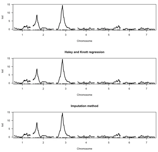
scanone いう関数 用い SIM 行う

3 ^{方法 結果 ほ あ} Fig. 1 ^{こ こ 高密}

配置さ い 間 在 QTL 計算方法 違う 計算

3 手法 違い 出 考え そこ こ 以降 計算 3 手法 中

計算速 速い _hk 用い 解析 行う

# calculate the probabilities of genotypes at equal-spaced potisions on the map interval <- 2 # 2 cM intervals

cross <- calc.genoprob(cross, step = interval)

# preparation for the imputation method. it takes some time cross <- sim.geno(cross, step = interval, n.draws = 1000)

# determine environment env.id <- 16

# interval mapping with the EM-algorithm

out.em <- scanone(cross, pheno.col = env.id + 1, method = "em") plot(out.em)

# large QTL are detected on the 2nd and 3rd chromosome

# interval mapping with the Haley and Knott regression

out.hk <- scanone(cross, pheno.col = env.id + 1, method = "hk") plot(out.hk)

# interval mapping with the imputation method

out.imp <- scanone(cross, pheno.col = env.id + 1, method = "imp") plot(out.imp)

par(mfrow = c(3,1)) # plot 3 figures simultaneously to make comparison plot(out.em, main = "EM-algorithm")

plot(out.hk, main = "Haley and Knott regression") plot(out.imp, main = "Imputation method")

# difference between methods is quite small

par(mfrow = c(1,1)) # reset the number of figures plotted simultaneously to 1

Fig. 1. 3 異 手法 単純 ン ッ ン 結果 SIM 横軸 第 〜７染

色体 置 縦軸 _LOD 値 大 いほ そ 場所 _QTL あ 可能性 高い こ

手法間 違い ほ 見 い

LOD ^{値 大 さ 基} QTL ^{検出 い値 決 い値}

決 前 QTL 表示 LOD 値 断さ QTL

表示さ い値 決 並べ え検 permutation test 行う 並べ

え検 表現型 無作 並び え _QTL 解析 繰 返 行う 無作 並

び え こ 遺 伝 子 型 表 現 型 対 応 関 係 撹 乱 さ 本 来

い QTL 関 情報 消失 う 逆 見 並び え 行 検

出さ う _LOD 値 偽物 _QTL 偽陽性 起因 考え こ

0 5 10 15

EM-algorithm

Chromosome

lod

1 2 ³ 4 ^{5 6} 7

0 5 10 15

Haley and Knott regression

Chromosome

lod

1 2 ³ 4 ^{5 6} 7

0 5 10 15

Imputation method

Chromosome

lod

1 2 ³ 4 ^{5 6} 7

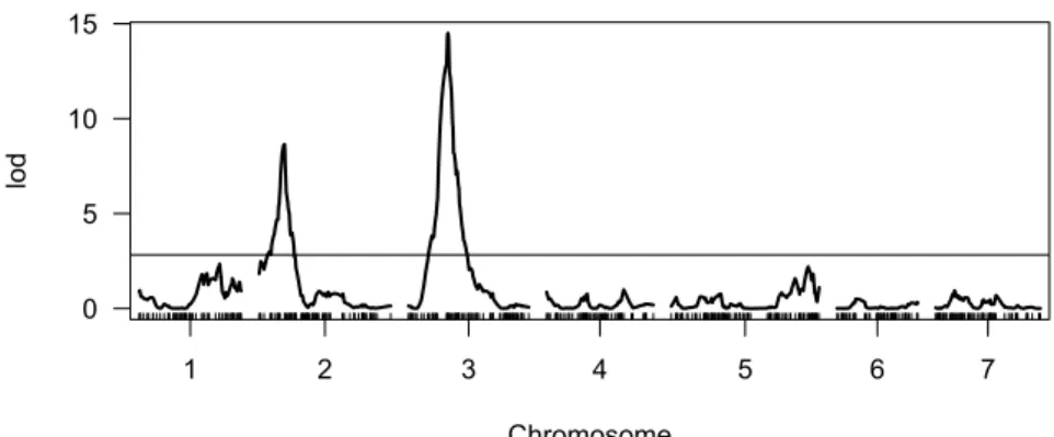
う 基 並び え 毎 QTL 解析 行い 染色体全域 中 LOD 大

値 記録 こ 複数回 例え 1,000 回 繰 返 こ QTL 無

い場合 _LOD 値 布 経験的帰無 布 求 い値 例え こう 得

経験的帰無 布 5% 等 設 例え 5％ 設 QTL 無い

誤 偽 QTL 検出 う確率 ノ 全体 5% う 設 さ こう

求 い値 _LOD 値 う 意 求 こ 場合

2 QTL 領域 検出さ Fig. 2

Fig. 2. 単純 ン ッ ン SIM 結果 線 並べ え検 求 LOD

値 _LOD 値 線 あ 置 _QTL 在 考え 領域

0 5 10 15

Chromosome

lod

1 2 ³ 4 ^{5 6} 7

# show the list of QTL detected by the hk regression summary(out.hk)

# perform a permutation test to get a threshold for LOD score to detemine QTL regions operm.hk <- scanone(cross, pheno.col = env.id + 1, method = "hk", n.perm = 1000)

# show the threshold obtained from the permtation test summary(operm.hk, alpha = 0.05)

# with this threshold, it is expected to detect non-QTL as QTL at the 5% probability

# show the QTL result figure with the threshold plot(out.em)

abline(h = summary(operm.hk, alpha = 0.05))

# close up one chromosome chr.id <- c(2,3)

plot(out.em, chr = chr.id)

abline(h = summary(operm.hk, alpha = 0.05))

# show the list of QTL detected with the threshold summary(out.hk, perms = operm.hk, alpha = 0.05)

検出さ QTL 効果 推 行 う makeqtl 関数 検出さ QTL 置

遺 伝 子 型 抜 出 そ 独 立 変 数 明 変 数 表 現 型 従 属 変 数 被 明

変数 回帰 述 い値 従う _{2 QTL} 検出さ _{Fig. 3} こ

QTL 効果 誤差 比べ そ 大 さ あ 大 く無く 回帰 析 け F 検 結果

意 い

Fig. 3. 単純 ン ッ ン SIM 検出さ 2 QTL

200

150

100

50

0

Chromosome

L o ca ti o n (cM)

1 2 ³ 4 ^{5 6} 7

Genetic map

Q1

Q2

# estimate QTL effects

temp <- summary(out.hk, perms = operm.hk, alpha = 0.05) # output the list of significant QTL qtl <- makeqtl(cross, chr = temp$chr, pos = temp$pos, what = "prob")

res <- fitqtl(cross, qtl = qtl, get.ests = T, method = "hk")

# show the result

plot(qtl) # plot the location(s) of QTL

summary(res) # summary of fitting significant QTL

# QTL effects are not so strong, and the result of F-test for QTL are not significant...

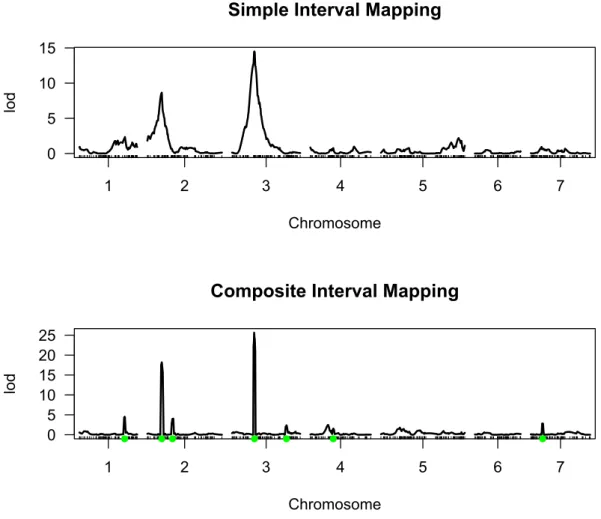
ン ッ ン ッ ン composite interval mapping CIM 行

う CIM 共変量 数 ここ 7 設 解析 窓 大 さ そ 窓 中

共変量 配置 い ここ ₅ 設 指 解析 行う必要 あ _SIM

CIM 結果 図示 比較 前者 比べ後者 QTL 置 解像 高いこ

Fig. 4 こ CIM 共変量 用い こ 注目 い 場所以外 置 い

QTL ^{影響 込 こ そ 引 起こ 変動 押さえ込 こ 注}

目 い 場所 あ QTL 明瞭 捉え う こ

SIM 様 並べ え検 行 決 い値 用 意 QTL 検出さ

い ここ 時間 節約 並び え ₁₀ 回 繰 返 い い 実際

100 回 繰 返 必要 あ

# perform the composite interval mapping with the Haley and Knott regression n.covar <- 7

window.size <- 5

outcim.hk <- cim(cross, pheno.col = env.id + 1, method = "hk", n.marcovar = n.covar, window = window.size)

# compare the results between SIM and CIM par(mfrow = c(2,1))

plot(out.hk, main = "Simple Interval Mapping") plot(outcim.hk, main = "Composite Interval Mapping") add.cim.covar(outcim.hk, col = "green")

par(mfrow = c(1,1))

# The resolution of CIM is much higher than SIM

# determine the threshold for QTL detection

opermcim.hk <- cim(cross, pheno.col = env.id + 1, method = "hk", n.marcovar = n.covar, window = window.size, n.perm = 10)

# With larger number of permutations, you can get a more accurate result.

# show the threshold obtained from the permutation test summary(opermcim.hk, alpha = 0.05)

# show the list of QTL detected with the threshold summary(outcim.hk, perms = opermcim.hk, alpha = 0.05)

# no QTL is significant...

Fig. 4. 単純 ン ッ ン SIM ン ッ ン ッ ン CIM

比較 _{CIM QTL} 置 推 さ

後 単純 ン ッ ン 用い 複数 QTL 間 交互作用 検出

行 う ここ _{2 QTL} 間 _scantwo 関数 索 並び え

検 結果 第 2 第 3 染色体 QTL 間 意 あ いう結果 得

2 QTL 時検出 場合 述 並べ え検 い値 決 こ

本 並べ え検 得 い値 基 く 第 ₂ び第 ₃ 染

色体間 意 検出さ

0

5

10

15

Simple Interval Mapping

Chromosome

lo d

1 2 ³ 4 ^{5 6} 7

0

5

10

15

20

25

Composite Interval Mapping

Chromosome

lo d

1 2 ³ 4 ^{5 6} 7

以 R 用い QTL 解析 方法 関 明 終わ あ ここ 2 番目 環境

い 解 析 行 異 環 境 計 測 さ 結 果 う 変 化

う _env.id いう変数 ₂ 以外 値 解析 繰 返 実行 解

析 設 例え CIM 際 共変量 数や窓 変化さ こ 得

結 果 変 化 示 少 変 更 解 析 行 い

い 発見 あ う

# scan two QTL interactions (epistasis)

out2.hk <- scantwo(cross, pheno.col = env.id + 1, method = "hk")

# show the result of the scanning plot(out2.hk)

## perform a permutation test to get a threshold for LOD score to determine epistasis operm2.hk <- scantwo(cross, method="hk", n.perm=100)

# show the threshold obtained from the permtation test summary(operm2.hk, alpha = 0.05)

# show the list of epistasis detected with the threshold summary(out2.hk, perms = operm2.hk, alpha = 0.05)

# one epistasis between the 2nd and 3rd chromosomes is significant

応用編 １ レポート課題

遺伝子連鎖地図

1. ^{#76 表 基 い 遺伝子 A-B 間 い 対数尤 組換え価 r 関数}

ln L ( r ) 書 そ _r 尤推 量 求 さい 式 基

遺伝子 _{A-C, B-C} 間 い 組換え価 求 さい

2. A-B, A-C, B-C 間 Haldane 地図距離 Kosambi 地図距離 ン ン単

求 さい log 計算 google 例え ln(0.3) 検索

0.3 ^{自然対数 計算}

3. ^{遺伝子 A B C 順 並 い 考え 妥当 う}

QTL 解析

4. ^{#58 示 F2 集団 離 考え 遺伝子 A, B 間 地図距離}

3cM あ A 2cM 置 B 1cM 置 置 QTL い

遺伝子型 _aaBb 個体 _{i QTL} 遺伝子型 _{QQ, Qq, qq} 確率 _p

_p

p

求 さい ここ 値 各地図距離 対応 組換え価 用

い さい _r

= 0.029 地図距離 3cM , r

=0.020 地図距離 2cM , r

=0.010 地

図距離 _1cM

5. ^{問 4 個体 i マーカー遺伝子型が aaBb い 表現型値 y}

^{1.2 あ}

今 #59 示 _µ =0.0, a =1.0, d =0.5, ^σ

=0.5 あ 場合

い 考え 場合 個体 _{i QTL} 遺伝子型 _{QQ, Qq, qq} 表現型 _y

_1.2 確率

#60 求 さい

QTL 解析の実習

6. ^{授業 16 環境 計測さ 収量 う 16 番目 env.id =16 い 解析}

16 番目 環境 似 環境 似 い い環境 い QTL 解析

行い そ 結果 比較 う

環境間 収量 類似性 環境間 相関係数 決 う

環境間 相関関係 cor(cross$pheno)定 求 こ

Env16 ^{正 相関 大 い環境 相関} 0 ^{近い環境 負 相関 大 い 負}

値 0 隔 い 環境 3 環境 い QTL 解析 行い そ 結果 比

較 う

収量 類似性 _QTL 解析 結果 う 関係 あ う

＜提出の仕方＞

以 い 方法 構い

電子 本文 内容 書く

PDF 作成 電子 添付

MS ⁻ Word ^{作成 電子 添付}

〜 い 方法 作成 iwata.report@gmail.com 送

さい 自動 理 送 返さ

＜期限

2016 年 12 23 日