プレゼンテーション１（マクロ第１章） ゼミナール kurosawalab

N.GREGORY MANKI W

macroeconomics 4 ^th edition

Chapter 4 : Economic growth ^Ⅰ

4-0 I ntroduction

4-1 The Accumulation of Capital 4-2 The Golden Level of Capital 4-3 Population Growth

4-4 Summary

04AK865

Yuusuke Souma

2005/ 05/ 17

4-0 I ntroduction

Difference in the Standard of living

Difference in the Standard of Living 1999~ 2002

[ ]

順 位 国 名 1 9 9 9 年 ァ 0 0 0 年 ァ 0 0 1 年 ァ 0 0 ァ 年

1 セ ブ 4 6 ウ 5 ア 4 4 6 ァ 1 4 4 9 0 5 4 6 ウ ァ ァ

ァ ー ア 5 5 ァ ェ ア ウ ア ア 9 ア ウ ェ 1 ア 4 ァ ァ ア 4

ア イ ア 6 0 6 0 ア ア 5 ァ 9 ア 4 ァ 1 6 ア ウ ア ェ 5

4 メ ア ァ ェ 9 0 ア 4 4 ウ ア ア 5 0 0 4 ア 5 ェ 9 ア

5 ー ア ァ 5 ェ 6 ァ 9 ウ 6 6 ァ 9 ェ ァ 6 ア ァ ア 6 6

6 日 本 ア 5 ア ア 6 ア ウ 4 0 ェ ア ァ ウ 4 5 ア 1 ァ ウ ウ

ウ イ ァ 5 ア 5 9 ァ 4 ェ ウ ウ ァ 6 5 5 5 ア 1 ァ 4 ァ

ェ イ ァ 9 9 4 ェ ァ 9 9 0 ア ァ ウ 1 5 5 ァ 9 1 ア ア

9 イ ァ 5 0 0 1 ァ 4 5 ア 6 ァ 4 ア 1 6 ァ 6 5 1 ァ

1 0 ァ 5 ァ 1 ア ァ ア ア 1 ウ ァ 4 0 5 0 ァ 6 0 ウ 6

ァ 1 ニ ュ ー ー 1 4 ェ 9 ウ 1 ア 4 ウ 5 1 ア ァ 0 ウ 1 5 0 5 5

ァ ァ ャ 1 1 6 1 6 1 0 ア 9 6 1 0 6 ウ 6 1 ァ 1 ア ウ

ァ ア 1 1 5 1 ァ 1 0 6 ァ ウ 1 1 0 0 ア 1 ァ 1 ァ ェ

ァ 4 韓 国 ェ ウ 4 6 9 ェ 5 6 9 0 6 ウ 1 0 0 5 1

ァ 5 コ 5 ア 5 0 5 0 0 ァ 5 5 ウ ウ 6 ウ ェ ァ

ァ 6 ー 4 ウ ウ 6 4 6 6 ア 5 1 9 9 6 6 ア ウ

ァ ウ メ コ 4 9 4 ア 5 ェ ウ ェ 6 ァ 1 1 6 ァ 4 6

ァ ェ ア 6 ウ 5 ア 5 5 ェ ア ウ ェ 1 4 9 ウ 0

ァ 9 コ ァ ウ 4 ウ ァ 9 ァ ア ァ 0 9 6 ァ 5 9 5

ー 4 0 1 1 4 0 ウ 6 4 5 5 ウ …

資 料 内 閣 府 経 済 社 会 総 合 研 究 所 国 民 経 済 計 算 年 報

原 資 料G D タ 及 び 為 替 ー O E C D " M a i ポ E c マ ポ マ m i c ジ ポ d i c a t マ r s " ( ァ 0 0 ア 年 1 1 月 版 )

一 部 国 に つ い ジ M F " ジ ポ t e r ポ a t i マ ポ a l F i ポ a ポ c i a l S t a t i s t i c s " ( ァ 0 0 ア 年 1 1 月 版 ) 人 口 ジ M F " ジ ポ t e r ポ a t i マ ポ a l F i ポ a ポ c i a l S t a t i s t i c s " ( ァ 0 0 ア 年 1 1 月 版 )

注 記 1 . 日 本 国 民 経 済 計 算 部 推 計 値

ァ . 順 位 ァ 0 0 ァ 年

ア ー ァ 0 0 ァ 年 ー 未 入 手 あ

出 展 経 済 要 覧 成 ６ 版 　 　 成 ６ ６ 月 日 発 行

編 集 ： 内 閣 府 経 済 社 会 総 合 研 究 所 　 発 行 ： 独 立 行 政 法 人 国 立 印 刷 局

諸 国 一 人 当 国 内 総 生 産 ( 名 目 Ｇ ) ( 米 表 示 ： 暦 年 )

4-0 I ntroduction

Solow Growth Model

„

^Solow

Growth Model

• Saving

• Population growth

• Technological progress

1) Robert Merton Solow 1924 ^‐

Affect the level of an economy

’

and it

’

4-1.1 The Accumulation of Capital

The Supply and Demand for Goods

„ The Supply of Goods and the Production Function

)

,

( K L

F

Y ₌

K: Capital L: Labor

„ The Solow model assumes that production fuction has constant returns to scale.

)

,

( zK zL

F

zY ₌

both capital and labor by z, we also multiply the amount

of output by z.

4-1.1 The Accumulation of Capital

The Supply and Demand for Goods

„

The Production Function

Output per

worker, y

Capital per worker, k

1

MPK

Output, f(k)

Diminishing marginal product

)

(

)

1

(

)

1

,

(

)

(

)

1

,

/

(

/

)

,

(

k

f

k

f

MPK

k

F

y

k

f

y

L

K

F

L

Y

L

K

F

Y

−

+

=

=

=

=

=

y: Y/ L k: K/ L

MPK: Marginal Product of Capital

Figure4-1: The Production Function

4-1.1 The Accumulation of Capital

The Supply and Demand for Goods

„ The Demand for Goods and the Consumption Function

The per-worker version of the national income identity for the economy

sy

i

i

y

s

y

y

s

c

i

c

y

=

∴

+

−

=

−

=

+

=

)

1

(

)

1

(

c : consumption per worker

i : investment per worker

s : saving rate

consumption saving

y: income

I nvestment = Saving

4-1.2 The Accumulation of Capital

Growth in the Capital Stock and the Steady State

Economy ’ s Output

Capital Stock

Key

Determination

∵

Capital stock can change over time.

Economic Growth

„ Growth in Capital Stock

4-1.2 The Accumulation of Capital

Growth in the Capital Stock and the Steady State

)

(

)

( k y f k

sf

i

sy

i _{= ⇔ =} ^∵ ₌

c= f(k)-sf(k)

i y

Output, f(k)

I nvestment, sf(k) Output

per worker, y

Capital per worker, k

Figure4-2: Output, Consumption and I nvestment

„ Output, Consumption and I nvestmemt

4-1.2 The Accumulation of Capital

Growth in the Capital Stock and the Steady State

Figure 4-3 Depreciation

Depreciation, ^δｋ

Capital

per worker, k Depreciation

per worker,^δ

Depreciation: The wearing out of old capital

Depreciation causes the capital stock to fall

δ：Depreciation Rate

„ Depreciation

4-1.2 The Accumulation of Capital

Growth in the Capital Stock and the Steady State

:

)

(

δ

δ

δ

k

k

sf

k

k

i

k

−

=

Δ

−

=

Δ

Depreciation Rate

i= sf(k)

Figure 4-4

I nvestment, Depreciation, and the Steady State

Capital per worker, k I nvestment and

Depreciation

K1 k K2

δ

δ

i2

i=

^δ

Depreciation, ^δk

I nvestment, Sf(k)

⊿ _k

„ Steady State

Steady State

4-1.3 Approaching steady state:

A Numerical Example

„ We assume production function is .

_{Y = K}

_L

9

1 . 0

3 . 0 ) (

) ( 0

) (

) (

2 / 1

2 / 1

2 / 1 2 / 1

2 / 1 2 / 1

=

=

=

−

=

−

= Δ

=

=

=

=

=

k k k

s k

f k

k k

sf

k k

sf k

k y

k y

L K L

Y

L L K

L Y

L K

Y

δ

δ ^δ

Y δｋ ⊿

：

：

：

：

∞

0 . 1 4

; 1 . 0

; 3 . 0

; _{= = =}

= ^{k s k}

y _δ

☆

^⊿

4-1.3 Approaching steady state:

A Numerical Example

I nvestment & Depreciation per worker

Capital per worker, k

Output, f(k)

2 0

lim 1

2

' 1

2 / 1

=

=

=

∞

→

_k

y k

k

y

k

4-1.3 Approaching steady state:

How Saving Affect Growth

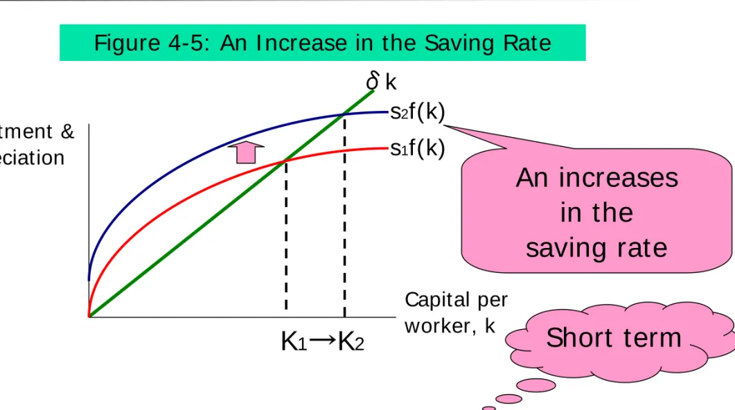
Figure 4-5: An I ncrease in the Saving Rate

I nvestment & Depreciation

Capital per worker, k

s¹f(k)

K¹ K²

s²f(k) δ_k

An increases in the

saving rate

Higher Saving Faster Growth

Short term

4-2.1 The Golden Rule Level of Capital:

Comparing Steady State

Figure 4-7: Steady-State Consumption _{c y i} i c y

−

= +

=

f(k* ): output

k* : capital per worker i=^δk* : investment

& depreciation

*

*) (

*

*

k k

f c

i y c

δ

−

=

−

=

Steady-state output and depreciation

Steady-state capital per worker,k*

Steady-state Output, f(k* )

Steady-state depreciation (and investment) ^δｋ*

K* ^gold

c* gold

Maximum distance

MPK=^δ MPK-^δ= 0

δ

=

*) ( ' k f

4-2.2 The Golden Rule Level of Capital :

Finding the Golden Rule Steady State: A Numerical Number

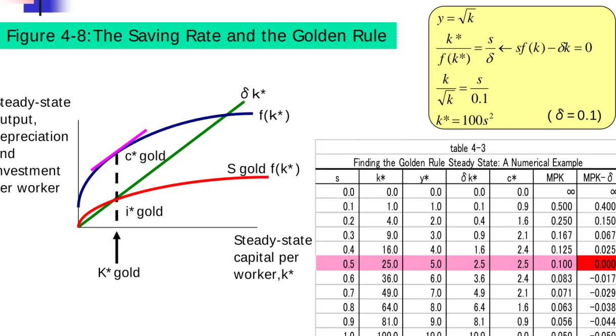
Figure 4-8: The Saving Rate and the Golden Rule

Steady-state output,

depreciation and

investment per worker

Steady-state capital per worker,k*

δｋ_*

K* gold c* gold

i* gold

f(^ｋ* )

S gold f(k* )

* * δ * * PK PK δ

∞ ∞

A

100 2

*

1 . 0

0 )

*) ( (

*

s k

s k k

k k

s sf k

f k

k y

=

=

=

−

←

=

=

δ δ

(^δ= 0.1)

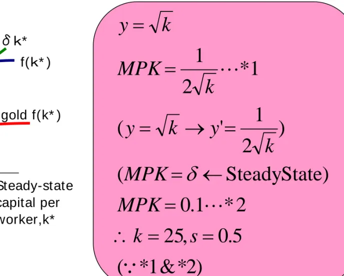
4-2.2 The Golden Rule Level of Capital :

Finding the Golden Rule Steady State: A Numerical Number

Figure 4-8: The Saving Rate and the Golden Rule

Steady-state output,

depreciation and

investment per worker

Steady-state capital per worker,k*

δｋ_*

K* gold c* gold

i* gold

f(^ｋ* )

S gold f(k* )

) 2

*

& 1

* (

5 . 0 ,

25

2

* 1 . 0

State) Steady

(

2 ) ' 1 (

1 2 *

1

Q

L L

=

=

∴

=

←

=

=

→

=

=

=

s k

MPK MPK

y k k

y MPK k

k y

δ

4-2.3 The Golden Rule Level of Capital :

The Transition to the Golden Rule Steady State

Figure 4-9: Reducing Saving When Starting With More Capital Than in the Golden Rule Steady

State

Figure 4-10: I ncreasing Saving When Starting With Less Capital Than in the Golden Rule

Steady State

t⁰

The saving rate is increased. Output,y

Consumption, c

I nvestment, i

t⁰ Time

The saving rate is reduced. Output,y

Consumption, c

I nvestment, i

Time

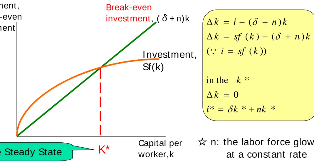
4-3.1 Population Growth :

The Steady State with Population Growth

Figure 4-11: Population Growth in the Solow Model

I nvestment, break-even investment

K*

Break-even

investment, (^δ+ n)k

I nvestment, Sf(k)

The Steady State

Capital per worker,k

*

*

*

0

* in the

)) ( (

) (

) (

) (

nk k

i k

k k sf i

k n k

sf k

k n i

k

+

=

= Δ

=

+

−

= Δ

+

−

= Δ

δ

δ δ Q

☆ n: the labor force glow at a constant rate

4-3.2 Population Growth :

The Effects of Population Growth

Figure 4-12: The I mpact of Population Growth

(^δ+ n²)k

k²*

I nvestment, break-even investment

k¹*

I nvestment, Sf(k)

Capital per worker,k

(^δ+ n¹)k

An increase in the rate of population growth

from n¹ to n²

k¹* k²* y* = f(k* )

Down

n MPK

n MPK

k n k

f c

i y c

=

−

+

=

+

−

=

−

=

δ^δ

δ ^{) *} (

*) (

*

Maximizes consumption

4-4.1 Summary

„ The solow growth model shows that in the long run, an economy’s rate of saving determines the size of its capital stock and thus its level of production. The higher the rate of saving, the higher the stock of capital and the higher the level of output.

„ I n the solow model, an increase in the rate of saving causes a period of rapid growth, but

eventually that growth slows as the new steady- state is reached. Thus, although a high saving rate yields a high steady-state level of output, saving by itself cannot generate persistent economic growth.

4-4.1 Summary

„ The level of capital that maximizes steady-state consumption is called the Golden Rule Level. I f an economy has more capital than in the Golden Rule steady state, then reducing saving will increase

consumption at all points in time. By contrast, if the economy has less capital of Golden Rule steady state, then reaching the Golden Rule requires increased

investment and thus lower consumption for current generation.

4-4.1 Summary

„ The solow model shows that an economy

’

determination of the standard of living. The higher the rate of population growth, the lower the level of output per worker.

出展：BIS 74th Annual Report (1 April 2003 - 31 March 2004) (Bank for International Settlements)

各国の貯蓄率