Numerical studies on the matrix model and
the expanding universe
Yuta Ito
)octor of Philosophy
)epartment of Particle and Nuclear Physics
School of High Energy Accelerator Science
SO0EN)AI (The Graduate University for
Advanced Studies)
Numerical studies on the matrix model
and the expanding universe
Yuta Ito
Department of Particle and Nuclear Physics,
Graduate University for the Advanced Studies (SOKENDAI), Tsukuba, Ibaraki, 305-0821, Japan
Abstract
In this thesis I study the dynamics of the space-time in the matrix models using numerical simulations. Recent studies on the Lorentzian type IIB matrix model show that (3+1)d space-time emerges dynamically from (9+1)d space-time predicted by superstring theory, which indicates the birth of the (3+1)d universe in the string theory. In order to investigate what happens at late times, I study the two simplified Lorentzian type IIB matrix models. We find that the emergent space expands exponentially at early times, which changes into a power-low behavior t1/2 with respect to time t at late times. This is reminiscent of the expanding behavior in the inflation and the Friedmann-Robertson- Walker universe in the radiation dominated era, respectively. Moreover, I investigate the infrared cutoff dependence of the expanding behavior in these models. For the simplified model, it turns out that the infrared cutoff effects disappear for a certain region of the cutoff parameter in the infinite volume limit.
On the other hand, I investigate the dimensionality of emergent space by the toy model of the Euclidean type IIB matrix model which has a spontaneous breaking of rotational SO(4) symmetry. From the complex Langevin approach, I show that introducing extra mass parameters in the Dirac operator extends the range of applicability of the method, which enable us to observe the spontaneous breaking of SO(4) symmetry. Moreover, I show that the result obtained by extrapolating the parameters to zero is consistent with the one obtained by another method.
Contents
1 Introduction 3
2 Review of the type IIB matrix model 6
3 Lorentzian version of the type IIB matrix model 12
3.1 Brief review of the Lorentzian type IIB matrix model . . . 13
4 Expanding behavior of the Universe 18 4.1 The simplified model for early times . . . 19
4.2 The simplified model for late times . . . 21
4.2.1 Properties of the bosonic model for N < Nc . . . 22
4.2.2 Properties of the bosonic model for N ≥ Nc . . . 23
5 The IR cutoff dependence of the expanding behavior 28 5.1 Generalization of the form of the IR cutoffs . . . 29
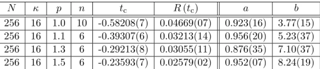
5.2 The p dependence of R (t) . . . 30
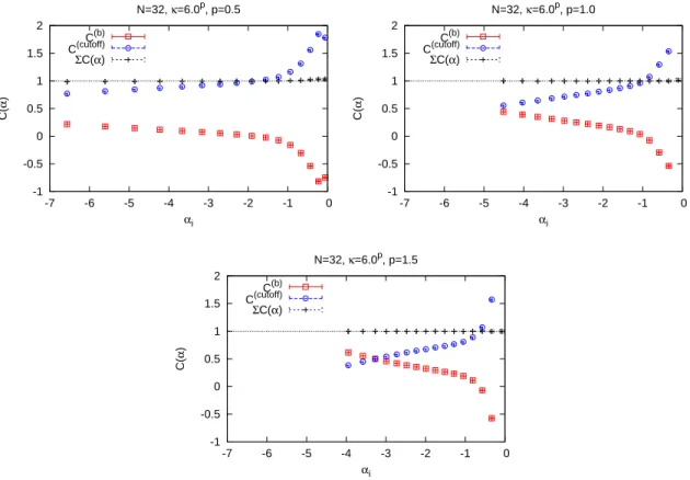
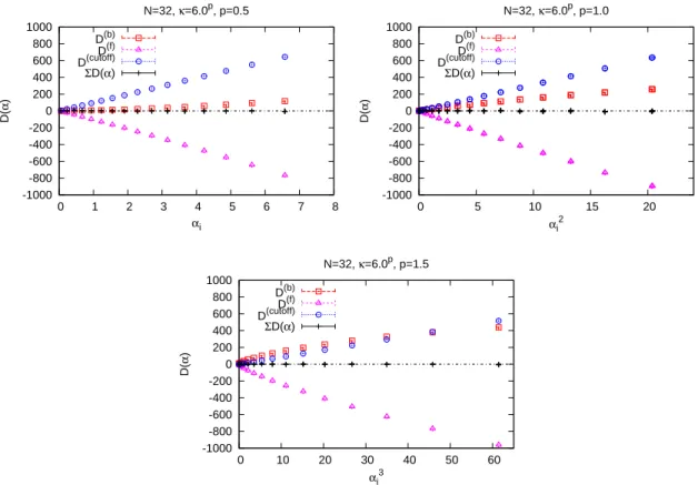
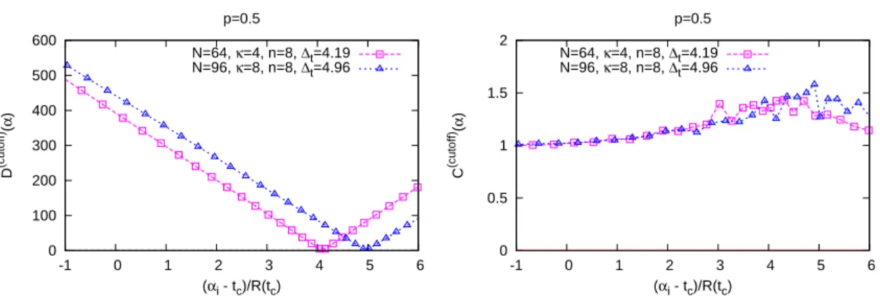
5.3 The Schwinger-Dyson equations in the simplified model . . . 31
6 The matrix model with SO(4) rotational symmetry 43 6.1 The definition of the toy model of the Euclidean type IIB matrix model . . . 44
6.2 Brief review of the complex Langevin approach . . . 48
6.3 The application to the complex action case . . . 49
6.4 Application of the complex Langevin method to the matrix model . . . 53
7 Summary and discussion 62
A Details of Monte Carlo simulation 65
B Results for the (5+1)D version of the bosonic model 67
C The differences between two simplified models 70
D Review of stochastic quantization and the Langevin equation 72
E The result for the another fermion mass term 78
1 Introduction
The Standard Model is extremely successful in understanding quantum field theory of fun- damental interactions and it can explain the experimental observations except for a few important remaining problems. In particular, lattice gauge theory has been established as the non-perturbative approach for studying physics of the strong interaction. The numerical study by the lattice gauge theory is actually the powerful approach to understanding the physics in the strong coupling region where perturbative approach is not applicable. On the other hand, describing the quantum gravity has not been achieved yet. However, the de- scription of quantum gravity is necessary to understanding dynamics of the early universe in which macroscopic description of gravity as general relativity breaks down due to the cosmic singularity. As a most promising candidate of quantum gravity theory, the string theory has been studied for a long time. However, superstring theory requires the space-time to be ten dimensional whereas our universe is four dimensional.
In fact, one can obtain four-dimensional space-time by compactifying the extra dimen- sions with various ways, which allows too many vacua giving four-dimensional low energy effective field theories with various gauge symmetries. Nevertheless, there is no guiding prin- ciple to pick up one vacuum from those vacua as far as one deals with superstring theory perturbatively. It is therefore necessary to consider superstring theory non-perturbatively.
As a non-perturbative formulation of superstring/M theory, matrix models were proposed. They can be obtained by dimensionally reducing the ten-dimensionalN = 1 super Yang-Mills theory to d = 0 [1], d = 1 [2] and d = 2 [3]. The matrix models can naturally describe the many-body system of strings.
The type IIB matrix model [1] is one of these proposals corresponding to the d = 0 case mentioned above, whose action can be derived from the Schild type world-sheet action of type IIB superstring by the matrix regularization. The important feature of this model is that the space-time does not exist a priori and is described dynamically as the eigenvalue distribution of the ten bosonic matrices. In this context, the idea of emergent gravity has been pursued [4–11] in the gauge theories on the non-commutative space which appear from the type IIB matrix model for a particular class of backgrounds [12–15]. Until recently, this model was studied after making a Wick rotation [16–29] because the partition function of the Euclidean model obtained in this way was shown to be finite [30,31]. However, the Euclidean model is not suitable for studying the real time dynamics because the time coordinate is treated as purely imaginary. Moreover, it is known that the Wick rotation is more subtle in quantum gravity theory than in quantum field theory at the non-perturbative level [32,33]. Indeed a recent study using the Gaussian expansion method suggests that the emergent space-
time in the Euclidean matrix model does not seems to be four-dimensional space-time [34]. On the other hand, the Lorentzian version of the type IIB matrix model has been studied using Monte Carlo simulation for the first time in ref. [35]. Unlike the Euclidean case, one has to introduce the infrared cutoffs in both the temporal and spatial directions in order to make the partition function finite. Although such a subtlety remains (it will be discussed in detail later), the Lorentzian matrix model is suitable for studying real-time dynamics. The eigenvalue distribution of the matrix representing the time coordinate can extend to infinity owing to the existence of supersymmetry, and dominant configurations of spatial matrices obtained by Monte Carlo simulation have a very nontrivial structure. This structure enables us to naturally extract the time evolution from the matrices. It turned out that the large-N scaling behavior is observed, and surprisingly, the SO(9) rotational symmetry of the 9d space is spontaneously broken down to SO(3) at some critical time, after which only three out of nine spatial directions start to expand. This emergence of 3d space indicates the birth of the three-dimensional universe in the string theory. It should be emphasized that the dimensionality of the space-time is determined uniquely by the non-perturbative dynamics of superstring theory in contrast to the perturbative superstring theory in which consistent vacua can have various space-time dimensionality.
As another important property of the Lorentzian IIB matrix model, it is expected that the classical approximation becomes valid at late times since each term in the action becomes large as the expansion of the “universe” proceeds, which enables us to to investigate possible behaviors at late times [36–40]. A general prescription to construct solutions to the classical equations of motion was given in ref. [37]. One can actually construct classical solutions corresponding to an expanding (3+1)d universe, which naturally solve the cosmological con- stant problem [37]. As a closely related progress, it was found that matrix configurations with intersecting fuzzy spheres in the extra dimensions can accommodate the standard model fermions [41–47]. In fact, it is known that the classical equations of motion of the matrix model have infinitely many solutions [37]. Therefore, in order to determine which classical so- lution is actually realized at late times, we need to study the time-evolution of the “universe” at least for a sufficiently long time by performing Monte Carlo simulation.
One can also study the qualitative behavior of the expanding 3d space in a long time evolution using the simplified models of the Lorentzian type IIB matrix model [48–50]. These models are obtained by using an approximation, which captures important properties of the original model at early times and at late times. This simplification and the usage of a large- scale parallel computer enable us to perform Monte Carlo simulation with much larger matrix size.
The first simplified model describes the early time behaviors of the original model [49].
With the matrix size N≤ 256, we observed a clear exponentially expanding behavior, which is reminiscent of the inflation. Monte Carlo studies of the original model with N = 24 [48] yielded results consistent with this observation. The second simplified model describes the late time behaviors of the original model, which is merely a bosonic model defined by omitting the fermionic matrices [50]. Unlike in the case of the original model, it turns out that the eigenvalue distribution of the temporal matrix has a finite extent without introducing an IR cutoff in the temporal direction due to the absence of supersymmetry. In spite of this, we find that the properties of the model changes drastically at the critical N = Nc, and one can extract the meaningful time-evolution for N ≥ Nc. Moreover, the model suggests that the exponential expansion terminates at some point in time and changes into the power-law t1/2 expansion which is consistent with the expanding behavior for the Friedmann-Robertson- Walker universe in the radiation dominated era. These results indicate that the exponential expansion of the space suggested in the original model actually ends at some point in time and turns into a power law similarly to the bosonic model. This would imply that the number of e-foldings is determined dynamically in the Lorentzian type IIB matrix model.
Let us recall that these interesting observations are obtained from the Lorentzian type IIB matrix model, which is regularized by infrared cutoffs. However, unlike in quantum field theories, it is not obvious that the effects of IR cutoffs disappear in the infinite volume limit because the extent of space-time is given by the dynamics of the model. Therefore we consider the IR cutoffs deformed with a parameter and study how it affects the expanding behavior in the simplified model. We found that the expanding behavior becomes universal for a certain range of the cutoff parameter. This suggests that the IR cutoff effects disappear for such a parameter region. We also found that this suggestion are supported by the analysis using the Schwinger-Dyson equation, in which the terms arising from the IR cutoffs decrease as N is increased for the same range of the cutoff parameter.
In this thesis, we also discuss the Euclidean version of the type IIB matrix model. In the Euclidean model the complex fermion determinant causes the sign problem which makes numerical studies difficult. As we mentioned earlier, there are several proposals to overcome this problem. Especially, the recent studies on the complex Langevin approach [51] and the Lefschetz thimble approach solve the sign problem for several simple cases [53–59]. One of the issues in the complex Langevin method we consider in this thesis is that the condition for which the method works is not understood very well. However, recent studies revealed certain criteria to justify the method, and in order to satisfy the criteria, one can consider an improvement called by the “gauge cooling”. It is known that the complex Langevin method (CLM) in fact becomes successful at some parameter region of QCD at finite density and the related Random Matrix theory.
In this thesis we consider a matrix model which is expected to undergo a spontaneous breaking of the rotational SO(4) symmetry. This model is considered as a simplified model of the Euclidean type IIB matrix model. In application of the complex Langevin approach to this simplified matrix model, it turned out that the gauge cooling for justifying the method does not work well enough. Therefore, in addition to the gauge cooling, we introduced the mass parameter mf to the fermion action to improve the method further. After taking the mf → 0 limit, we have shown that the SO(4) symmetry actually breaks spontaneously down to SO(2).
The rest of this paper is organized as follows. In section 2 we review the definition of the type IIB matrix model. In section3 we briefly review the definition and some important properties of the Lorentzian type IIB matrix model. In section 4 we define the simplified models, and present results obtained by direct Monte Carlo studies. In section5 we discuss the dependence of the expanding behavior of space-time on the IR cutoffs in the simplified model. In section 6 we study the Euclidean matrix model, in which we investigate the spontaneous breaking of rotational symmetry in the simplified model using the complex Langevin approach. Section7 is devoted to a summary and discussions.
2 Review of the type IIB matrix model
I briefly introduce the type IIB matrix model we consider in this paper. The model was proposed as a non-perturbative formulation of superstring theory, which is defined by dimen- sional reducing the 10d N = 1 SYM theory to zero-dimension. On the other hand, one can show that the model can be derived from the world-sheet action of the type IIB superstring by applying the matrix regularization. Moreover, the model naturally seems to describe the many-body system of strings by embedding them to matrix degrees of freedom. In what follows, I show that the action of the type IIB matrix model can be derived from the Shild type world-sheet action of the type IIB superstring.
The action of the type IIB matrix model is given by
S = 1
g2Tr (
[Aµ, Aν] [Aµ, Aν] + 1 2ΨΓ¯
µ[A µ, Ψ]
)
, (2.1)
where Aµ(µ = 0, . . . , 9) are the N× N Hermitian matrices. Γµare the 10d gamma matrices and Ψα(α = 1, . . . , 16) are the 10d Majorana-Weyl spinors which are also N× N Hermitian matrices. Therefore the action has the SO(9,1) symmetry.
Then, we show that the action (2.1) can be derived from the Green-Schwartz action for
the type IIB superstring
SGS=−T
∫ d2σ
(√
−12Σ2+ iϵab∂aXµ
(¯
θ1Γµ∂bθ1+ ¯θ2Γµ∂bθ2) + ϵabθ¯1Γµ∂aθ1θ¯2Γµ∂bθ2 )
, (2.2) where T is the tension of a string and σa(a = 1, 2) is the world-sheet coordinate. θ1 and θ2 are the 10d Majorana-Weyl spinors which have the same chirality in 10d space-time since we are considering the type IIB superstring. Σµν is defined by
Σµν = ϵabΠµαΠνb ,
Πµa = ∂aXµ− i¯θ1Γµ∂aθ1+ i¯θ2Γµ∂aθ2 . (2.3) Note that the action (2.1) is defined after taking the analytic continuation θ2 → iθ2.
One can show that the action (2.1) has the 10 dimensionalN = 2 supersymmetry δSU SYθ1 = ϵ1,
δSU SYθ2 = ϵ2,
δSU SYXµ = i¯ϵ1Γµθ1− i¯ϵ2Γµθ2 (2.4) and the κ-symmetry
δκθ1 = α1 , δκθ2 = α2 ,
δκXµ = i¯θ1Γµα1− i¯θ2Γµα2 , (2.5) where α1 and α2 are defined by
α1 = (1 + ˜Γ)κ1 , α2 = (1− ˜Γ)κ2 ,
Γ =˜ 1
2
√
−12Σ2
ΣµνΓµν . (2.6)
κ1 and κ2 are local parameter of the Majorana-Weyl spinors depending on the world-sheet coordinate σa. One can show that ˜Γ2= 1, from which it turns out that α1and α2 have only a half degree of freedom of θ1 and θ2. Therefore by fixing the gauge of the κ-symmetry, one can reduce the d. o. f. of θ1 and θ2 by half. Since the chirality of θ1 and θ2 are same, the
Lorentz symmetry is preserved even after the gauge fixing. Now, let us choose the gauge of the κ symmetry so that
θ1 = θ2 = ψ . (2.7)
Then the action (2.1) becomes
S˜GS=−T
∫ d2σ
(√
−1 2σ
µνσ
µν+ 2iϵab∂aXµψΓ¯ µ∂bψ )
, (2.8)
where
σµν = ϵab∂aXµ∂bXν . (2.9)
One can see that the action (2.8) still has the N = 2 supersymmetry by defining a new supersymmetric transformation so that the gauge fixing condition (2.7) is preserved as
δθ1 = (δSU SY + δκ) θ1, δθ2 = (δSU SY + δκ) θ2,
δXµ = (δSU SY + δκ) Xµ, (2.10)
and in order to satisfy δθ1 = δθ2 we set κ1 and κ2 as
κ1 = −ϵ
1+ ϵ2
2 ,
κ2 = ϵ
1− ϵ2
2 . (2.11)
Then, by introducing new parameters ξ and ϵ as
ξ = ϵ
1+ ϵ2
2 ,
ϵ = ϵ
1− ϵ2
2 , (2.12)
we can rewrite theN =2 supersymmetry using ξ and ϵ as δ(1)ψ = − 1
2
√
−12σ2
σµναΓµνϵ ,
δ(1)Xµ = 4i¯ϵΓµψ , (2.13)
and
δ(2)ψ = ξ ,
δ(2)Xµ = 0. (2.14)
Furthermore, we rewrite the Nambu-Goto type action (2.8) to the Schild type action. In order to do this, we introduce the Poisson bracket
{X, Y } ≡ √1gϵab∂aX∂bY, (2.15)
where √g is the world-sheet density defined by the metric gab on the world-sheet. Using the Poisson bracket, the action (2.8) can be written as
SSchild=
∫
d2σ[√gα( 1 4{X
µ, Xν}2
− i 2ψΓ¯
µ{Xµ, ψ}
)
+ β√g ]
. (2.16)
One can show that the above action is equivalent to the Nambu-Goto type action (2.8). In fact, the equation of motion for √g is given by
−14αg1(ϵab∂aXµ∂bXν
)2
+ β = 0 . (2.17)
Then one obtains
√g = 1 2
√α β
√
(ϵab∂aXµ∂bXν)2. (2.18) By substituting (2.18) to the Shild type action (2.16), one obtains the action as
∫ d2σ
(
√αβ√(ϵab∂aXµ∂bXν)2− i 2αϵ
ab∂
aXµψΓ¯ µ∂bψ
)
, (2.19)
which is equivalent to (2.8) up to the normalization.
Note that theN = 2 supersymmetry is realized for the Schild type action (2.16) as δ(1)ψ = −1
2{Xµ, Xν} Γ
µνϵ ,
δ(1)Xµ = i¯ϵΓµψ , (2.20)
and
δ(2)ψ = ξ ,
δ(2)Xµ = 0 . (2.21)
Here, one can formally consider the quantization of the action (2.16) with the path integral formalism as
Z =
∫
D√gDXDψ eSSchild . (2.22)
In addition to theN = 2 SUSY, the action (2.16) has the diffeomorphism invariance for the world-sheet such as
δdψ = ϵa∂aψ , δdXµ = ϵa∂aXµ ,
δd√g = ϵa∂a√g . (2.23)
Note that we assume here that the measure of the path integral (2.22) is invariant under the transformation (2.23). For instance, one considers to fix the gauge for which √g is constant all over the world-sheet. Therefore the infinitesimal transformation of √g in (2.23) becomes
δd√g = ϵa∂a√g = 0 . (2.24)
The solution of the above differential equation is given by ϵa= √1
gϵ
ab∂
bρ (2.25)
using the arbitrary function ρ (σa). Then substituting (2.25) to (2.23) gives the “area pre- serving diffeomorphism” as
δdψ = {ψ, ρ} , δdXµ = {ψ, Xµ} ,
δd√g = 0 . (2.26)
In particular, it satisfies the w∞-algebra which is described by the Poisson bracket. One considers to regularize the path integral (2.22), in which one regularizes the w∞-algebra with the SU(n) algebra. When n is sufficiently large, one can approximate the Poisson bracket and the integral with respect to the world-sheet coordinate by the commutator and the trace of matrices
{ , } → −i [ , ] , 1
2π
∫
d2σ → Tr . (2.27)
In this context, the bosonic fields Xµand fermionic fields ψ become n×n Hermitian matrices and the properties for the Poisson bracket
∫
d2σ√g{X, Y } =
∫
d2σ ∂a(ϵabX∂bY)= 0 ,
∫
d2σ√gX{Y, Z} =
∫
d2σ√gZ{X, Y } (2.28)
are replaced by the relations
Tr ([X, Y ]) = 0 ,
Tr (X [Y, Z]) = Tr (Z [X, Y ]) . (2.29) Therefore, by replacing the Poisson bracket and the integral in (2.16) and (2.22) by the commutator and the trace, one obtains the action and partition function of the type IIB matrix model as
SIKKT = α (
−1
4Tr [AµAν]
2−1 2Tr
(¯
ψΓµ[Aµ, ψ]) )
+ 2πβTr1 , (2.30)
Z =
∞
∑
n=0
∫
dAdψ e−SIKKT, (2.31)
where we denote the n× n Hermitian matrices by Aµ. The integral with respect to √g is replaced by the summation over n which represents the area of the world-sheet. The measure in the path integral (2.31) is the Haar measure which is defined as
dA = ∏
µ
(
∏
i
d (Aµ)ii )
∏
i>j
dRe (Aµ)ijdIm (Aµ)ij
,
dψ = ∏
α
(
∏
i
d (ψα)ii )
∏
i>j
dRe (ψα)ijdIm (ψα)ij
. (2.32)
One can easily see that the action (2.30) also has the N = 2 supersymmetry. According to the rule (2.27), the supersymmetry transformation for the type IIB matrix model is given as
δ(1)ψ = i
2[Aµ, Aν] Γ
µνϵ ,
δ(1)Aµ = i¯ϵΓµψ , (2.33)
and
δ(2)ψ = ξ ,
δ(2)Aµ = 0 . (2.34)
The type IIB matrix model can describe states including more than one string while the Schild action represents the action for one string. In fact, by considering block diagonal configurations, the action (2.30) can be decomposed with the direct sum of block matrices, in which each block represents one string state described by the Schild type action. In that case, off-diagonal blocks can be interpreted to represent interactions between corresponding two strings. Thus, the matrix model is expected to describe the second quantization of string theory.
Note that the term proportional to Tr1 in (2.30) and the summation over n in the path integral (2.31) do not exist in the original action of the type IIB matrix model. This can be interpreted that (2.30) is the effective action obtained by integrating out some sub-matrices. Therefore when one regards βTr1 as a chemical potential for matrix size n, one can interpret the partition function (2.31) as the micro canonical ensemble version of the type IIB matrix model.
3 Lorentzian version of the type IIB matrix model
As was explained in section2, the type IIB matrix model describes states of more than one string or D-brane as the d.o.f. of matrices. The eigenvalues of matrices describe the positions of D-branes and their distribution can be regarded as the extent of emergent space-time from 10d space-time. Thus, the type IIB matrix model would explain how 4d space-time emerges from the 10d space-time required by superstring theory.
There are many studies on the type IIB matrix model, in which the model have been studied after making the Wick rotation. In the Euclidean model, the partition function turns out to be well-defined and one can deal with it numerically. In that case, the model has SO(10) symmetry. However, it has not been shown how the dimensionality is chosen. In particular, the study using the Gaussian expansion method suggests that the emergent space is three-dimensional rather than four-dimensional.
On the other hand, the Lorentzian version of the type IIB matrix model has been studied in ref. [35]. In the Lorentzian case, the time coordinate is treated as real and the model is suitable for investigating real time dynamics. Although the action becomes imaginary, it turned out that the imaginary action can be approximated by a delta function, which enables
us to deal with the Lorentzian model numerically. One has to introduce IR cutoffs in practice since the action is unbounded. As a result of numerical analysis, it turned out that the only three out of nine spatial directions start to expand at some point in time-evolution. In what follows, I will briefly review the definition of the Lorentzian type IIB matrix model and the result mentioned above.
3.1 Brief review of the Lorentzian type IIB matrix model
The action of the Lorentzian type IIB matrix model is given by [1]
S = Sb+ Sf , (3.1)
Sb = 1
4g2Tr ([Aµ, Aν] [A
µ, Aν]) , (3.2)
Sf = − 1 2g2Tr
(
Ψα(CΓµ)αβ[Aµ, Ψβ]) , (3.3) where the bosonic N×N matrices Aµ(µ = 0, . . . , 9) and the fermionic matrices Ψα(α = 1, . . . , 16) are both traceless and Hermitian. Γµare 10D gamma-matrices after the Weyl projection and C is the charge conjugation matrix. The “coupling constant” g is merely a scale parameter in this model since it can be absorbed by rescaling Aµ and Ψ appropriately. The indices µ and ν are contracted using the Lorentzian metric ηµν = diag (−1, 1, . . . , 1). The Euclidean version can be obtained by making the “Wick rotation” A0 = iA10, where A10 is supposed to be Hermitian.
The partition function for the Lorentzian version is proposed in ref. [35] as Z =
∫
dAdΨ eiS (3.4)
with the action (3.1). The “i” in front of the action is motivated from the fact that the string world-sheet metric should also have a Lorentzian signature. By integrating out the fermionic matrices, we obtain the Pfaffian
∫
dΨ eiSf = PfM (A) , (3.5)
which is real unlike in the Euclidean case [29]. Note also that the bosonic action (3.2) can be written as
Sb= 1
4g2Tr (FµνF
µν) = 1
4g2
{−2Tr (F0i)2+ Tr (Fij)2} , (3.6) where we have introduced the Hermitian matrices Fµν = i [Aµ, Aν]. Since the two terms in the last expression of eq. (3.6) are non-positive definite and have opposite signs, Sb is not
positive semi-definite. Therefore it is not bounded from below.
In order to make the partition function (3.4) finite, one needs to introduce infrared cutoffs in both the temporal and spatial directions, for instance, as
1
NTr (A0)
2 ≤ κN1 Tr (Ai)2 , (3.7)
1
NTr (Ai)
2 ≤ Λ2 . (3.8)
It is important to confirm that the IR cutoffs can be removed in the infinite volume limit, which is discussed in Section (5).
In the present work, it is important to understand the reason why we need to introduce the cutoff (3.7) in the temporal direction. Note first that one can use the SU (N ) symmetry of the model to bring the temporal matrix A0 into the diagonal form
A0 = diag (α1, . . . , αN) , where α1<· · · < αN . (3.9)
By “fixing the gauge” in this way, we can rewrite the partition function (3.4) as
Z =
∫ 9
∏
i=1
dAi
N
∏
k=1
dαk∆(α)2PfM (A) eiSb , ∆(α)≡
N
∏
a>b
(αa− αb) , (3.10)
where ∆(α) is the van der Monde determinant. The factor ∆(α)2 in (3.10) appears from the Fadeev-Popov procedure for the gauge fixing, and it acts as a repulsive potential between the eigenvalues αk of A0. Here we consider a situation in which the eigenvalues of A0 are well separated from each other. Then the action S = Sb+ Sf can be expanded as
Sb = − 1
2g2(αa− αb)
2|(Ai)ab|2+· · · , (3.11) Sf = − 1
2g2(Ψα)ba(αa− αb) (CΓ
µ)
αβ(Ψβ)ab+· · · , (3.12) omitting the sub-leading terms for large|αa− αb|. Integrating out Ai at one loop neglecting the zero modes corresponding to diagonal elements, we obtain ∆(α)−18 for the one-loop potential of αk which acts as a attractive force between αk. On the other hand, integrating out Ψα at one loop similarly, we obtain ∆(α)16. Thus we find that the potential between αiis canceled exactly at the one-loop level. This is actually a consequence of supersymmetry [1] of the model (3.4). Owing to this property, the eigenvalue distribution of A0 extends to infinity even for finite N if the cutoff (3.7) were absent.
In fact, after some manipulation and rescaling of Aµ, we can rewrite the partition function
(3.4) as Z =
∫
dA PfM (A) δ( 1
NTr (FµνF
µν)
) δ( 1
NTr (Ai)
2− 1 )
θ (
κ− 1
NTr (A0)
2
)
=
∫ N
∏
a=1
dαa
d
∏
i=1
dAi∆2(α) PfM (A) δ( 1
NTr (FµνF
µν)
)
×δ( 1
NTr (Ai)
2− 1
) θ
( κ− 1
NTr (A0)
2
)
, (3.13)
where θ (x) is the Heaviside step function. This form allows us to performing Monte Carlo simulation of the Lorentzian model without the sign problem unlike the Euclidean model.1
Let us note first that the integrand of the partition function (3.4) involves a phase factor eiSb. As is commonly done in integrating oscillating functions, we introduce a convergence factor e−ϵ|Sb| and take the ϵ→ 0 limit after the integration.
Then the partition function can be rewritten as
Z =
∫ dA
∫ Λ2 0
dr δ( 1
NTr (Ai)
2− r )
θ (
κr− 1
NTr (A0)
2
)
eiSb−ϵ|Sb|PfM , (3.14) where κ and Λ are the cutoff parameters introduced in (3.7) and (3.8), respectively. Rescaling the variables Aµ→ r1/2Aµ in the integrand, we get
Z =
∫
dA PfM(A) f(Sb) δ( 1
NTr (Ai)
2− 1
) θ
( κ− 1
NTr (A0)
2
)
, (3.15)
where the function f (Sb) is defined by
f (Sb)≡
∫ Λ2 0
dr r9(N2−1)−1er2(iSb−ϵ|Sb|) . (3.16) Note that f (Sb) is a complex-valued function with the property f (−Sb) = f (Sb)∗. For
|Sb| ≪ Λ14, the function can be well approximated by
f (Sb) ≈
∫ Λ2
0
dr r9(N2−1)−1
= 1
9(N2− 1)(Λ
2)9(N2−1) . (3.17)
For|Sb| ≳ Λ14, the phase of the integrand in (3.16) starts to oscillate violently in the region
1Strictly speaking, the Pfaffian PfM in (3.13) can change its sign, but it turned out that configurations with positive Pfaffian dominate at large N .
r ≳ 1/√|Sb|, and hence the integral decreases rapidly in magnitude for increasing |Sb|. In particular, the asymptotic behavior of f (Sb) for|Sb| ≫ Λ14 can be estimated as
f (Sb) f (0) ∼
1 2Γ
( 9 2(N
2− 1)
)
|Sb|−92(N2−1)· 9(N2− 1)(Λ2)−9(N2−1)
= Γ( 9 2(N
2− 1) + 1
) ( 1 Λ4|Sb|
)92(N2−1)
(3.18)
by deforming the integration contour in (3.16). Recalling eq. (3.2), the condition |Sb| ≪ Λ14
for (3.17) can be rewritten as
1
NTr (FµνF
µν)
≪
4g2
N Λ4 . (3.19)
Therefore, assuming that the right-hand side N Λ4g24 of (3.19) becomes small at large N , we may make a replacement
f (Sb) =⇒ δ( 1
NTr (FµνF
µν)
)
(3.20) up to a normalization constant. Rescaling the variables Aµ→ Aµ/L, we arrive at eq. (3.13). Within the above approximation, the parameter L simply sets the scale of the model, and we may use L = 1 without loss of generality.
It turns out that one can extract a time-evolution from configurations generated by sim- ulating (3.13). A crucial observation is that the spatial matrices Ai have a band-diagonal structure in the SU(N ) basis in which A0 has the diagonal form (3.9). More precisely, there exists some integer n such that the elements of spatial matrices (Ai)ab for |a − b| > n are much smaller than those for|a − b| ≤ n. Based on this observation, we may naturally consider n× n matrices
(¯
Ai)IJ(t)≡ (Ai)ν+I,ν+J , (3.21)
as representing the state of the universe at time t, where I, J = 1, . . . , n and ν = 0, 1, . . . , N− n. The time t in (3.21) is defined by
t = 1 n
n
∑
I=1
αν+I (3.22)
corresponding to the n× n matrices ¯Ai. For example, we can define the extent of space at time t as
R2(t) =
⟨1 ntr
∑
i
(¯ Ai(t))2
⟩
, (3.23)
where the symbol tr represents a trace over the n× n block. We also define the “moment of inertia tensor”
Tij(t) = 1 ntr
(¯
Ai(t) ¯Aj(t)) , (3.24)
which is a 9× 9 real symmetric matrix. The eigenvalues of Tij(t), which we denote by λi(t) with the order
λ1(t) > λ2(t) >· · · > λ9(t) , (3.25)
represent the spatial extent in each of the nine directions at time t. Note first that the appearance of the gap between⟨λ3(t)⟩ and ⟨λ4(t)⟩ signals the spontaneous symmetry breaking of SO(9) to SO(3). Let us therefore define the separations dj(t) =⟨λj(t)⟩ − ⟨λj+1(t)⟩. Then we find that the symmetric phase can be characterized by d1(t) > d2(t) >· · · > d8(t), while
in the broken phase we find d2(t) < d3(t). Therefore we may define the critical time tc by the largest value of t′ such that d1(t) > d2(t) > · · · > d8(t) holds for t ≤ t′. Therefore the expectation values ⟨λi(t)⟩ tend to be equal in the large-N limit if the SO(9) symmetry is not spontaneously broken. This is the case at early times of the time-evolution. After a critical time tc, however, we find that three largest eigenvalues⟨λi(t)⟩ (i = 1, 2, 3) become significantly larger than the others, which implies that the SO(9) symmetry is spontaneously broken down to SO(3).
It would be interesting to study a long time-evolution of the model and see how the expansion of space proceeds. This requires very large matrices, which makes the simulation unfeasible. In the previous work [49], we studied a simplified model, in which the Pfaffian is replaced by the one-loop contribution ∆(α)16mentioned above. This replacement is expected to be valid at early times, where the expansion of space has not proceeded much and the leading term in (3.12) is indeed dominant. According to the argument below (3.12), the potential between the eigenvalues of A0 is canceled at one loop and hence the cutoff (3.7) in the temporal direction is needed in this simplified model as well as in the original model. On the other hand, this simplified model can be simulated with much less effort than the original model.2 In ref. [49] the (5+1)d version of the simplified model was studied with the matrix size N ≤ 64, and the SO(5) symmetry was found to be broken spontaneously down to SO(3) at some point in time similarly to the original model. Moreover, the expanding behavior of the 3D space turned out to be exponential,3 and no tendencies of slowing down were observed within the scaling region.
2In order to make one trajectory in the Hybrid Monte Carlo algorithm, the original model requires O(N5) arithmetic operations, whereas the simplified model requires only O(N3) arithmetic operations. The reason for this is that the number of iterations required for the convergence of the conjugate gradient method used to implement the effects of fermions grows as O(N2).
3This behavior is also confirmed with smaller matrix size N ≤ 32 with the aid of a renormalization group method developed in the same paper [49].
0 0.5 1 1.5 2 2.5
-2 -1 0 1 2
R(t)/R(tc)
(t-tc)/R(tc)
N=8 N=12 N=16 N=24 0.914+0.086exp(1.40t)
Figure 4.1: The extent of 9d space R (t) normalized by R (tc) is plotted against time (t− tc) /R (tc). The broken line is a fit to R (t) /R (tc) = a + (1− a) exp (bx) with x = (t− tc) /R (tc).
As I will show in the next section, analogous behaviors are also confirmed for the (9+1)d version of the simplified model. In the original model, on the other hand, the sub-leading term in the fermionic action (3.12) becomes important at late times as the expansion proceeds, and hence it can affect the expanding behavior.
4 Expanding behavior of the Universe
As I have explained in the previous section, the Lorentzian type IIB matrix model has the interesting property such that the spontaneous symmetry breaking from SO(9) to SO(3). Moreover, as shown in Fig. 4.1, it turned out that the emergent 3d space seems to expand exponentially. However, that expanding behavior is unclear since the time-evolution we have observed is too short to identify it while it is interesting to discuss relations to the inflation if the exponential expansion can be confirmed. Therefore, we consider simplified models of the original Lorentzian model in order to see qualitative expanding behavior in further time- evolution. In this section, we define two simplified models which are expected to describe the expanding behavior at early times and late times, and we discuss how the behaviors depend on such the region in the time-evolution.
4.1 The simplified model for early times
In the Lorentzian case, we have investigated the original type IIB matrix model only for N ≤ 24 since it takes enormous time to evaluate the Pfaffian.
As an approach to enlarge the matrix size, we consider to deal with the simplified model. We first consider a simplified model obtained by approximating the original model at early period in the time evolution as I will explain below [49]. We focus on approximating the fermion action to simplify the calculation of the Pfaffian. The fermion action (3.3) can be decomposed into two terms as
Sf ∝ Tr( ¯Ψα(Γ0)αβ[A0, Ψβ])+ Tr( ¯Ψα(Γi)αβ[Ai, Ψβ]). (4.1) Since the emergent space is not so large at early times, it is expected that the components of A0 are much larger than that of Ai. In such a situation, the contribution from the first term in (4.1) becomes dominant compared to one from the second term. Then we may merely omit the second term to obtain the simplified model for early times. After that, we can perform explicitly the integration with respect to the fermion matrices, which gives the Pfaffian as
PfM (A) ≃ ∆16(α) , (4.2)
where ∆ (α)≡∏i>j(αi− αj) is the van der Monde determinant. Thus the partition function of the simplified model for early times is given from (3.13) and (4.2) as
Z =
∫ 9
∏
i=1
dAi
N
∏
k=1
dαk∆18(α) δ (Sb) δ( 1 NTr(A
2i) − 1 )
θ (
κ− 1 NTr(A
20
) )
, (4.3)
where the extra factor ∆2(α) comes from the Fadeev-Popov procedure for the gauge fixing (3.9).
In the original Lorentzian type IIB matrix model, we have investigated the time-evolution of space-time with up to N = 24 [48], in which the exponential expansion of R (t) is not clear because we can observed only so short time-evolution. Moreover we have studied the 6d version of the simplified model with up to N = 64 [49], in which we have found that R (t) actually grows exponentially.
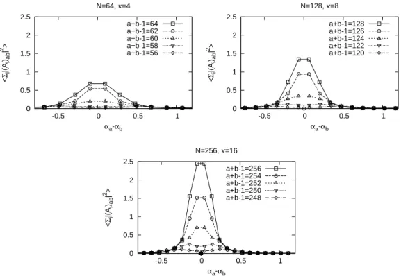
In order to explain how to determine values of the block size n introduced in (3.21), we plot the magnitude of the off-diagonal elements of Aifor N = 64, 128, 256 in Fig.4.2. We find that the magnitude decreases rapidly as one goes away from diagonal elements. Moreover, the magnitude scales only for sufficiently large |αa− αb|. From these observations, we identify the block size n as the number of points in the region where the off-diagonal elements do not
0 0.5 1 1.5 2 2.5
-0.5 0 0.5 1
<Σi|(Ai)ab|2>
αa-αb N=64, κ=4
a+b-1=64 a+b-1=62 a+b-1=60 a+b-1=58 a+b-1=56
0 0.5 1 1.5 2 2.5
-0.5 0 0.5 1
<Σi|(Ai)ab|2>
αa-αb N=128, κ=8
a+b-1=128 a+b-1=126 a+b-1=124 a+b-1=122 a+b-1=120
0 0.5 1 1.5 2 2.5
-0.5 0 0.5 1
<Σi|(Ai)ab|2>
αa-αb N=256, κ=16
a+b-1=256 a+b-1=254 a+b-1=252 a+b-1=250 a+b-1=248
Figure 4.2: The magnitude∑i|(Ai)ab|2 of the off-diagonal elements of Ai is plotted against the time separation αa− αb for N = 64, 128 and 256 with κ = 4, 8 and 16, respectively. The scaling is observed only for sufficiently large|αa− αb|. For N = 64, we find 6 points in the region in which the scaling behavior is violated. Analogous plots for N = 128, N = 256 are shown in the other panels, where we find 10 points in the non-scaling region.
0 0.02 0.04 0.06 0.08 0.1
-1.2 -1 -0.8 -0.6 -0.4 -0.2
<λi>
t N=128, κ=8.0, n=10
<λ1>
<λ2>
<λ3>
<λ4>
<λ5>
<λ6>
<λ7>
<λ8>
<λ9>
0 20 40 60 80 100
-1 -0.5 0 0.5 1 1.5 2 2.5 3 R2(t)/R2(tc)
(t - tc)/R(tc) N=64,κ=4,n=6 N=128,κ=8,n=10 N=256,κ=16,n=10
Figure 4.3: (Left) The nine eigenvalues of Tij(t) are plotted against time t for the simplified model with N = 128, κ = 8.0, n = 10 using the IR cutoffs (3.7) and (3.8). (Right) The extent of the space R2(t) normalized by R2(tc) is plotted against x = (t− tc) /R (tc) for the simplified model with N = 64 ,128 and 256 using the IR cutoffs (3.7) and (3.8) . The dashed line is a fit to R2(t) /R2(tc) = a + (1− a) exp (bx) with N = 256 for 0 ≤ x ≤ 1.3, which gives a = 0.89(3) and b = 4.0(3).
scale.
Once the block size n is determined in this way, we can obtain the time-evolution. We show here results for the 10d version of the simplified model with up to N = 256. In Fig.4.3 (Left), we plot the expectation values⟨λi(t)⟩ of the nine eigenvalues of Tij(t) with N = 128, from which we obtained the value of critical time as tc=−0.63108(7) for N = 128. Applying the same procedure to another N , we find that the large-N scaling becomes less clear due to the finite N effects. However, these finite N effects can be absorbed by adjusting the values of tc slightly from the one determined by the above argument.
Using tc determined in this way, we plot the extent of space R (t) normalized by R (tc) against t in Fig. 4.3 (Right), in which we find that the behavior of R2(t) at t > tc can be fitted well to an exponential function.
4.2 The simplified model for late times
In this subsection, we consider the second simplified model of the Lorentzian type IIB matrix model, which can be expected to describe the expanding behavior at late times. The model is defined as just a bosonic model in which the fermionic matrices are simply omitted. The partition function is given by
Z =
∫
dA eiSb . (4.4)
In section 3.1 I reviewed an argument for the necessity of the temporal cutoff in the original model and the simplified model for early times. In the present case of the bosonic
model (4.4), the same argument implies that one does not have to introduce the temporal cutoff (3.7), and that we only need the spatial cutoff (3.8). Corresponding to (3.13), we can study the bosonic Lorentzian type IIB matrix model by simulating
Z =
∫
dA δ( 1
NTr (FµνF
µν)
) δ( 1
NTr (Ai)
2− 1 )
(4.5)
=
∫ d
∏
i=1
dAi
N
∏
k=1
dαk∆2(α) δ( 1
NTr (FµνF
µν)
) δ( 1
NTr (Ai)
2− 1 )
, (4.6)
which requires computational efforts comparable to the simplified model for early times re- viewed in the previous section. We have used a large-scale parallel computer to simulate the model (4.6) with the matrix size up to N = 512, which enables us to investigate a long time-evolution. See AppendixA for the details of the simulation.
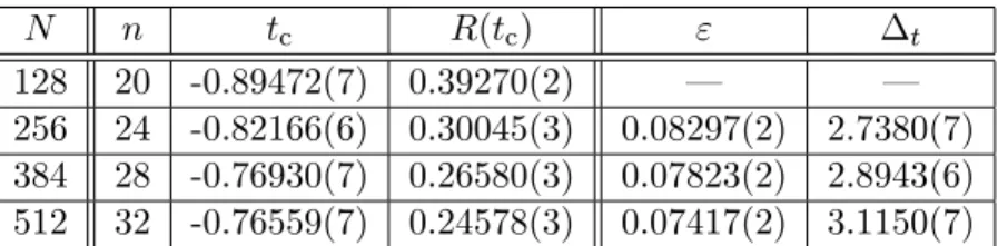
In order to show that there is no need to introduce temporal cutoffs in the bosonic model, we measure the quantity ⟨N1Tr (A0)2⟩, which represents the extent of the eigenvalue distribution of A0. As we mentioned above, it turns out that this quantity keeps to be finite in the model (4.6) although we do not introduce a cutoff in the temporal direction such as (3.7). In Fig.4.4(Left) we plot the results against N . At small N , it is almost independent of N . However, for N ≥ Nc= 112, it begins to increase linearly with N . At this time, the behavior for the spatial direction also drastically changes. In order to see its N dependence, we plot the expectation values ⟨λi(t)⟩ of the nine eigenvalues of Tij(t) evaluated at t = tpeak where R2(t) becomes maximum in Figure 4.4 (Right)4. For small N , there is no significant gap between the nine eigenvalues, whereas for N ≥ Nc, we observe a big gap between ⟨λ3(tpeak)⟩ and⟨λ4(tpeak)⟩. As was explained in previous section, this significant implies the spontaneous breaking of the rotational symmetry of the 9d space. We will see that the SO(9) symmetry is broken down to SO(3) after a critical time similarly to the original Lorentzian type IIB matrix model.
4.2.1 Properties of the bosonic model for N < Nc
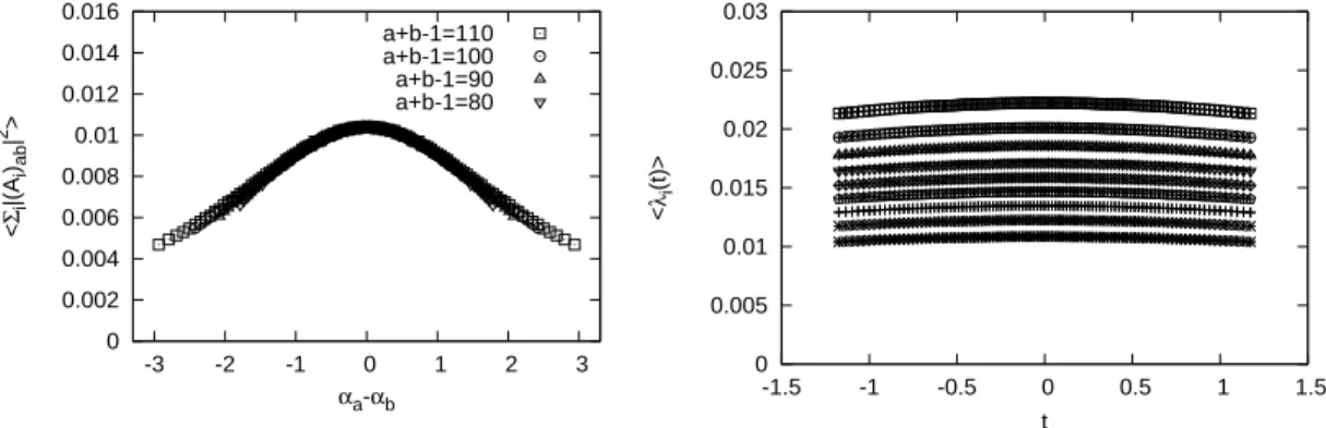
In this sub-subsection we discuss the properties of the bosonic model for N < Nc. In order to extract the time-evolution, we need to determine the block size n to be used in eq. (3.21). In Fig.4.5 (Left) we plot the magnitude of the off-diagonal elements of Ai against the time separation αa− αb for N = 110. The origin in the horizontal axis corresponds to the diagonal elements. We observe a nice scaling behavior for all the matrix elements. However, the magnitude falls off rather smoothly as one goes in the off-diagonal direction, which means
4In order to define R2(t) and Tij(t), we have to specify the block size n to be used in eq. (3.21). See sections4.2.1and4.2.2for the actual values of n used to obtain the results in Fig.4.4(Right).
0 2 4 6 8 10
0 100 200 300 400 500
<tr(A02)/N>
N 1/N trA02 (0.02475)*N -1.4601
0 0.1 0.2 0.3 0.4 0.5 0.6 0.7
0 100 200 300 400 500
<λi (tpeak)>
N
Figure 4.4: (Left) The extent ⟨N1Tr (A0)2⟩ of the eigenvalue distribution of A0 is plotted against N . (Right) The expectation values λi(t) of the nine eigenvalues of Tij(t) at t = tpeak are plotted against N . For N < Nc = 112, the nine eigenvalues are close to each other, whereas for N ≥ Nc, three out of the nine eigenvalues become much larger than the others. that the dominant matrix configurations do not have a band-diagonal structure.
In this situation, we cannot naturally define the block matrices (3.21) representing the state at each time and hence the notion of time-evolution becomes obscure. Indeed, we have shown that the temporal direction does not extend with N increased. Let us nevertheless try to extract the time-evolution using n = 14 as the block size, which is the value obtained for N = Nc = 112 in the way described in the next section. In Fig.4.5 (Right) we plot the expectation values ⟨λi(t)⟩ for N = 110. It turns out that there is only little t-dependence, and there is no clear gap between the eigenvalues for all t.
The situation for smaller N is similar to the N = 110 case. In Fig.4.6we plot the extent of space R2(t) as a function of t for N = 64, 96 and 110 obtained with the same block size n = 14. The dependence on N turns out to be modest.
4.2.2 Properties of the bosonic model for N ≥ Nc
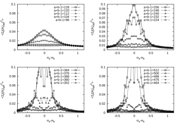
In this sub-subsection we study the properties of the bosonic model for N ≥ Nc. In Fig.4.7 (Left) we plot the magnitude of the off-diagonal elements of Ai for N = 128. We find that the magnitude decreases rapidly as one goes away from diagonal elements. Moreover, the magnitude scales only for sufficiently large |αa− αb|. From this observation, we identify the block size n as the number of points in the region where the off-diagonal elements do not scale. (In the present N = 128 case, we obtain n = 20. See below for more detail.)
Using the block size n determined in this way, we can obtain the time-evolution. In Fig. 4.7 (Right) we plot the expectation values ⟨λi(t)⟩ for N = 128. In contrast to the situation for N < Nc, we observe the spontaneous symmetry breaking from SO(9) to SO(3)