Market research and complementary advertising under
asymmetric information
Toshihiro Tsuchihashi∗† January 2010
Abstract
We consider whether a seller can benefit from price discrimination through market research in experience goods markets under bilateral asymmetric information. A low quality seller is likely to benefit from market research, while a high quality seller cannot improve her revenue by using market research alone. However, a synergy effect of the marketing mix exists, and the high quality seller can enjoy the synergy effect by combining advertising with market research. The availability of advertising and market research to both types of sellers results in a disappearance of information asymmetry and efficient trade.
1 Introduction
A variety of factors determine consumers’ willingness to pay (or perceived value) for products. When the consumers’ willingness to pay is not private information, firms try to infer the willingness to pay in order to be able to discriminate the price.1 Market research, such as group discussions, mail surveys and telephone interviews, serves this purpose and indeed is widely used. Sales in the business research industry in 2006 reached US$8232 million in the US (0.062% of GDP) and US$1380 million in Japan (0.028% of GDP) (Japan Market Research Association, 2008). If, in addition, product quality is private information of the firm, the firm may try to convey this information to consumers in order to avoid adverse selection problems.2
∗Graduate School of Economics, Hitotsubashi University; 2-1, Naka, Kunitachi, Tokyo 186-8601
†I am very grateful to Keizou Mizuno, Taiji Furusawa, Kazumi Hori, Hideshi Itoh, Daisuke Oyama and attendees at the Hitotsubashi Game Theory Workshop for helpful comments and suggestions. I am truly indebted to my adviser Akira Okada for his invaluable guidance. Any remaining errors are of course my own responsibility.
1The consumers’ willingness to pay can be estimated using information about the consumers’ purchasing behavior. Allenby and Rossi (1999) compare the empirical tools for estimating consumers’ willingness to pay. Besanko et al. (2003) note that firms may imperfectly classify consumers’ willingness to pay into segments when the firms can only obtain aggregate data on consumers’ heterogeneity.
2For example, price promotions and low-price strategies often lower the evaluation of products by consumers (Blattberg and Neslin 1990).
Advertising also serves this purpose. In fact, most firms involved in actual business transactions combine advertising with market research.
This paper studies a model of bilateral asymmetric information in order to explore the roles of market research and advertising as tools for eliciting the buyer’s and the seller’s private in- formation, respectively. We address the following two questions. First, under what conditions does market research increase seller revenue and improve market efficiency? Second, does rev- enue increase and market efficiency improve more by mixing advertising and market research? Whether to combine these two options or to use only one of them is also an important decision for the seller.
Specifically, we consider the following model. There is one seller and one buyer. The seller provides the product whose quality, either high (H) or low (L), is the seller’s private information. The buyer’s interest in the product, either high (H) or low (L), is the buyer’s private information. The buyer’s valuation of the product depends on both the product quality and his interest in the product. The seller’s valuation of the product is normalized to zero independently of the seller’s type, but the production cost is higher for H-seller than L-seller. The seller can use two marketing tools, market research (MR) and advertising (AD), to resolve the asymmetric information problem. The buyer’s interest in the product is perfectly conveyed to the seller through market research, while the product quality is perfectly conveyed to the buyer through advertising. We consider four cases: (1) neither MR nor AD is available to the seller, (2) only AD is available, (3) only MR is available, and (4) both MR and AD are available.
We obtain two results. First, the H-seller cannot benefit from price discrimination by using market research alone, even when its cost is zero. However, the L-seller can profitably use market research and discriminate prices, whenever the cost is sufficiently low. Observing a low price, the buyer would infer that the product quality is surely low. Thus, the H-seller could not offer a low price even if the seller knew that the buyer was an L-buyer, making market research useless for the H-seller. However, the L-seller offers a low price to the L-buyer since a sufficiently low price can bring positive profit to the L-seller, making market research useful for the L-seller. If, in addition, the probability of the buyer being the H-buyer is sufficiently high, market research improves market efficiency; i.e., increasing the probability of trading between
the seller and the buyer. Without market research, both types of sellers offer the high price, which is acceptable to only the H-buyer in this case. However, market research brings about trading between the L-seller and the L-buyer through the low price offered by the L-seller.
Second, the combination of market research and advertising creates a positive synergy effect on revenue, and the H-seller enjoys the synergy effect while the L-seller does not. By advertising the product quality, the H-seller can offer the low price without lowering the quality evaluation of the buyer in the case that the buyer’s type is low. This is the source of the synergy effect. However, the L-seller has no incentive to advertise the low quality; thus, the synergy effect does not exist for the L-seller.
This paper assumes that the seller can discriminate prices once the seller knows the buyer’s type. Price discrimination is widely studied in the literature of economics. Varian (1989) points out that the seller can always benefit from discriminating the prices in the market under unilateral asymmetric information; i.e., the buyer knows the product characteristics with certainty.3 However, he does not discuss the market under bilateral asymmetric information, which we focus on in this paper.
A huge literature on advertising exists. Since Nelson (1970, 1974) introduced the difference between consumption goods and experience goods, and discussed TV-commercial-type adver- tising as a signal of higher product quality to the buyer even though advertising is not directly informative in the experience goods markets, many papers discuss advertising as a signal of higher quality. However, few papers analyze free-sample-type advertising, which does not work as a signal but conveys the actual product quality to consumers. Moraga-Gonzalez (2000) examines the free-sample-type advertising as informative advertising and focuses on experience goods markets where advertising is informative and publicity expenses are not observable. As Moraga-Gonzalez (2000) discusses, whether advertising can work as a signal or convey direct information depends on the type of products in the market. For example, detailed information about the functions of personal computers or home electric appliances is disclosed on product websites. This detailed information can be considered as informative advertising.4
3Corts (1998) shows that, in imperfectly competitive oligopoly markets, it is ambiguous whether price dis- crimination gives the sellers higher profits or not under unilateral asymmetric information.
4Quality certification is similar to informative advertising. Biglaiser (1993) and Biglaiser and Friedman (1994) analyze the role of middlemen who can certify the product quality in the market under unilateral asymmetric information. They show that the middlemen can improve welfare in all equilibria in a general bargaining
This paper is organized in the following way. Section 2 presents the model. Section 3 analyzes the equilibria. Section 4 discusses the properties of marketing activities and the effect on market efficiency and sales. Section 5 provides some extensions and Section 6 concludes. All proofs are presented in the appendix.
2 The Model
There are four players: a seller, a buyer, an advertising agent and a market researcher. The seller provides a new product into the (experience goods) market. The buyer will at most purchase one unit of the product. The buyer’s payoff depends on both the product quality and his private interest in the product. The quality of the product has two possible types, either low (L) or high (H), which is the seller’s private information. The product quality i has a value θiS (θHS > θSL >0) to the buyer. We denote θS ∈ ΘS = {θLS, θSH}. We call the seller with the product quality i the i-seller. The prior probability of the H-seller is denoted by α ∈ (0, 1). The marginal cost of the product to the i-seller is denoted by ci, and cH > cL= 0 is assumed. We assume that the seller’s reservation value is normalized to zero.
The buyer’s interest has two possible types, either low (L) or high (H), which is the buyer’s private information. A level of interest j is represented by the value θBj (θHB > θBL > 0). We denote θB ∈ ΘB = {θLB, θHB}. We call the buyer with the interest j the j-buyer. The prior probability of the H-buyer is denoted by β ∈ (0, 1). We assume that the buyer’s payoff depends on both the product quality and his private interest in the product, which is denoted by V (θSi, θjB) = Vji. We assume VjH > VjL>0 for j = L, H and VHi > VLi >0 for i = L, H. For example, a buyer’s reservation value for a computer may be determined both by the computer’s intrinsic quality, reflecting features such as memory size and processor performance, and by his private interest in the computer depending on whether he frequently uses the computer or seldom. The advertising agent provides an advertising service (shortly, AD) for an advertising fee a, while the market researcher provides a market research service (shortly, MR) for a market research fee m. In the market, the seller can use AD and/or MR. When a trade occurs with
model when adverse selection is present. However, Lizzeri (1999) shows that the middlemen (which he calls intermediaries) may gain from the manipulation of information, resulting in imperfect product certification. This is the big difference between informative advertising and quality certification. Shavell (1994) proposes that market efficiency can be improved by the seller’s disclosure of the product quality.
price p and the seller uses both AD and MR, the i-seller receives the profit: p− ci
| {z }
revenue
− (a + m)
| {z }
marketing cost
,
and the j-buyer receives the payoff:
Vji− p.
The seller can make the product quality public information using AD, while the market re- searcher conveys the private interest of the buyer to the seller. Notice that the buyer cannot observe whether the seller uses MR or not.
The incomplete information game (Harsanyi, 1967–1968) has five stages.
Stage 1. The advertising agent and the market researcher independently choose their service fees, as take-it-leave-it offers.
Stage 2. The seller and the buyer privately know their types.
Stage 3. Knowing the product quality, the seller decides whether to use AD and/or MR. Stage 4. The seller assigns a price to the product, which is a take-it-leave-it offer to the buyer. Stage 5. Knowing a price and his interest in the product, the buyer decides whether to buy the product or not.
A strategy for the advertising agent is choosing an AD service fee a ∈ R+. A strategy for the market researcher is choosing an MR service fee m ∈ R+.
A (pure) strategy for the seller is a triplet s = (k, l, p). First, the seller decides whether to use AD or not, given her type and the AD fee, and it is formally described as a function k from ΘS× R+to {0, 1} where 0 means not using AD and 1 means using AD. Second, the seller decides whether to use MR or not, given her type and the MR fee, and it is formally described as a function l from ΘS× R+ to {0, 1}, where 0 means not using MR and 1 means using MR. Finally, the seller chooses a non-negative price given her type according to a function p from ΘS× ΘB to R+ when she uses MR, and a function from ΘS to R+ when she does not.
A strategy for the buyer is a pair b = (b0, b1) of decision rules to buy the product. In the case where the seller does not use AD, the decision rule b0 is given by a function from ΘB× R+
to {0, 1} where 0 means not buying and 1 means buying. In a case the seller uses AD, the decision rule b1 is given by a function from ΘB× ΘS× R+ to {0, 1}.
We analyze a perfect Bayesian equilibrium (PBE) of the game. A PBE of the game is represented by a profile (a∗, m∗, s∗, b∗, µ∗) of strategies and beliefs, where the buyer’s belief µ∗ is his probabilistic assessment of the seller’s type, given the price, and it is formally a function from R+ to the set of all probability distributions over the seller’s type set ΘS.5 We denote by µ(θiS|p) the probability that the buyer’s belief µ assigns to the i-seller conditional on observing price p. In what follows, we make the following assumption on the buyer’s belief.
Assumption 1 (Monotone beliefs) The buyer’s belief µ is monotone if there exists some ˆ
p∈ R+ such that, for some µ0 ≥ 0, the probability µ(θHS|p) satisfies:
µ(θSH|p) =
(µ0 if p ≥ ˆp
0 if p < ˆp. (1)
It is well known that many equilibria exist in general in signaling games with incomplete information.6 Monotone beliefs imply that the buyer’s subjective probability of the seller being a high type (H) is non-decreasing in price p. As noted by Fudenberg and Tirole (1983), the assumption of monotone beliefs means that higher prices would make the buyer perceive that he is facing a higher type seller. Monotone beliefs are intuitive and standard in the literature of sequential bargaining with asymmetric information. Without loss of generality, we adopt a step function instead of a continuous function as a monotone belief. A PBE outcome constructed under a step-function is preserved even if we adopt a continuous increasing function.
Definition 1 (Perfect Bayesian equilibrium) A profile (a∗, m∗, s∗, b∗, µ∗) of strategies and a belief is a perfect Bayesian equilibrium (PBE) of the game if (i) all four agents maximize their conditional expected payoffs given all available information,7 and (ii) the buyer’s belief µ∗ is monotone, and furthermore it obeys the Bayesian updating rule whenever it is possible. If not possible, the buyer’s belief may be arbitrarily selected, maintaining monotonicity.
5More precisely, the buyer’s belief includes his assessment of whether the seller uses MR or not. It is shown that a PBE of the model does not depend on this part of her belief.
6Nonmonotone beliefs induce a PBE in which any prices are equilibrium prices whenever they are not too high. To construct such a PBE, we consider the situation where a buyer identifies a seller of low quality with certainty for all prices except p∗, even though this situation is not realistic.
7Since the formulation of the maximization problem of an agent’s conditional expected payoff is standard, we omit it to avoid notational complexity.
The following three types of PBE may arise. A PBE is separating if different types of sellers offer different prices. In a separating PBE, the buyer can correctly infer the true product quality from the price. A PBE is pooling if all types of sellers offer the same price. In a pooling PBE, the buyer acquires no additional information on product quality from the price. A PBE is semi-separating if one type of seller offers at least two prices and another type of seller offers one of the prices. In a semi-separating PBE, the buyer who observes a price offered by both types of sellers cannot acquire any additional information on the product quality from the price, while the buyer who observes a price offered by only one type of seller can correctly infer the true product quality from the price. We basically consider pure strategy equilibria, but if they do no exist, then we consider mixed strategy equilibria.
3 Equilibrium
In this section, we consider the following four different games and characterize a PBE for each. (1) Neither AD nor MR is available (benchmark). (2) Only AD is available. (3) Only MR is available. (4) Both AD and MR are available.
Since the buyer’s optimal strategy is common in all four cases, we characterize it, first. Given the seller’s belief µ and price p, if the j-buyer buys the product, he obtains the expected payoff given by:
µ(θHS|p)VjH+ µ(θLS|p)VjL− p = EµVji− p.
Here, EµVji represents the j-buyer’s (expected) willingness to pay for the product under belief µ. It is clear that the optimal choice of the j-buyer is to buy the product if and only if p≤ EµVji.8 That is:
b∗j(p) =
(1 if EµVji≥ p 0 if EµVji< p.
We denote the j-buyer’s willingness to pay for the product under the initial belief by: EVji= (1 − α)VjL+ αVjH.
8We assume that the buyer buys the product if he is indifferent between buying and not buying.
Given the buyer’s optimal strategy, the seller will optimally choose a price from a closed interval [VLL, VHH]. The upper bound of the price VHH is the highest reservation value of the buyer; therefore, any price p > VHH is not acceptable to the buyer for any belief. The lower bound of the price VLL is the lowest reservation value of the buyer; therefore, the price p = VLL is accepted by both types of buyers for any belief. Any price p < VLL is, of course, accepted by both types of buyers, but the price brings a lower profit to the seller than price p = VLL; thus, any price p < VLL can never be optimal for the seller. Before proceeding in our analysis, we make some assumptions related to the buyer’s valuation function.
Assumption 2 (Buyer’s valuation).
VHH− VHL≥ VLH − VLL>0 (2)
cH > EVLi. (3)
Inequality (2) says that the increase of the payoff by switching from the low quality product to the high quality product is higher for the H-buyer than for the L-buyer. This implies that there is a positive interaction between product quality and the buyer’s interest for the buyer. Inequality (3) says that the L-buyer’s willingness to pay under the initial belief is less than the product cost of H-seller. Inequality (3) implies that trading with the L-buyer should result in a negative profit to the H-seller if the L-buyer keeps his initial belief, inducing inefficiency in trading under incomplete information. In other words, inequality (3) eliminates a case where both types of sellers offer the same price to the L-buyer under the initial belief. As we will see, AD and MR may eliminate the inefficiency.
3.1 Benchmark (Neither AD nor MR)
We first analyze the benchmark case where neither AD nor MR is available. The benchmark case involves one-shot bargaining with bilateral asymmetric information. In this case, we will prove that a separating PBE exists when β is smaller than the threshold β and that a pooling PBE exists when β is larger than the threshold ¯β. The two thresholds β < ¯β are defined by:
β= V
L L
VHH,
β¯= V
L L
EVHi . (4)
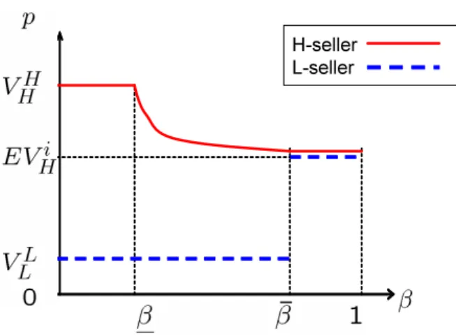
Suppose that the seller faces an H-buyer with probability β. Since βVHH = VLL, the L-seller is indifferent between offering the lowest price p = VLL, which is accepted with probability one, and the highest price p = VHH which, is accepted with probability β. If β < β, the L-seller prefers to offer the lowest price p = VLL. Suppose, however, that the seller faces the H-buyer with probability ¯β. Since ¯βEVHi = VLL, the L-seller is indifferent between offering the intermediate price p = EVHi which, is accepted with probability ¯β, and the lowest price p = VLL, which is accepted with probability one. If β > ¯β, the L-seller prefers to offer the intermediate price p = EVHi.
Proposition 1 (Separating PBE) If β ≤ β, there exists a unique PBE, which is separating. In equilibrium, the H-seller offers price p = VHH, while the L-seller offers price p = VLL. The price p = VHH is accepted by only the H-buyer, while the price p = VLL is accepted by both types of buyer. The buyer’s belief is given by:
µ(θSH|p) =
(1 if p ≥ VHH 0 if p < VHH.
If β ≤ β, the seller is likely to face the L-buyer, and thus both types of sellers would like to offer low prices that are acceptable to the L-buyer. If both types of sellers set different prices that they deem acceptable to the L-buyer, the buyer should be able to determine the product quality from the prices. In such a case, however, if the L-seller benefits from mimicking the H-seller’s price, thus different prices cannot exist. Suppose that both types of sellers set the same price, which is acceptable to the L-buyer. Inequality (4) implies, however, that this price results in a negative profit for the H-seller. Thus, the H-seller cannot trade with the L-buyer, and she is forced to assign a high price to the product, which is accepted by only the H-buyer, which results in a separating PBE. The separating PBE exhibits a standard adverse selection problem in which the H-seller cannot trade with the L-buyer.9
9Akerlof (1970) was the first to point out the adverse selection problem. Myerson and Satterthwaite’s (1983) well-known study shows that under bilateral asymmetric information, no mechanism can enforce trade whenever a seller and a buyer can benefit from the trade. In their model, the seller’s value is independent of the buyer’s. Chatterjee and Samuelson (1983), Manelli and Vincent (1995) and Lindsey et al. (1996) show that the same inefficiency exists when a buyer’s value is correlated with a seller’s, which is similar to the model in this paper.
Proposition 2 (Pooling PBE) If β ≥ ¯β, there exists a unique PBE, which is pooling. In equilibrium, both types of sellers offer price p∗ = EVHi, which is accepted by the H-buyer. The buyer’s belief is given by:
µ(θHS|p) =
(α if p ≥ p∗ 0 if p < p∗.
If β ≥ ¯β, the seller is likely to face the H-buyer, and thus both types of sellers would like to offer high prices that are acceptable to only the H-buyer. However, both sellers cannot offer different prices to target the H-buyer since the L-seller can benefit from mimicking the H-seller’s price without reducing the probability of trading. Thus, both types of sellers offer the same price acceptable to the H-buyer in equilibrium. Note that the H-seller can offer a low price acceptable to the L-buyer, but the low price brings a lower profit than the equilibrium price.
Since no pure strategy equilibrium exists for βin(β, ¯β), we seek mixed strategy equilibria.
Proposition 3 (Semi-separating PBE) If β < β < ¯β, there exists a unique PBE, which is semi-separating. In equilibrium, the H-seller offers price p = V
L L
β , while the L-seller mixes price p = V
L L
β with probability γ > 0 and p = VLLwith probability 1 − γ, where γ= α
1 − α·
βVHH − VLL VLL− βVHL. The equilibrium price p = V
L L
β is accepted by only the H-buyer, while p = VLL is accepted by both types of buyers. The buyer’s belief is given by:
µ(θSH|p) =
( α
α+(1−α)γ if p ≥ VLL
β
0 otherwise.
The equilibrium price p = V
L L
β offered by both types of sellers can be written as a function of β in the following way:
p(β) = α
α+ (1 − α)γV
H H +
(1 − α)γ α+ (1 − α)γV
L H =
1 βV
L L.
Notice that the price p decreases in β. Furthermore, p(β) = VHH, p( ¯β) = EVHi. Thus, the equilibrium price offered by the H-seller is continuous in β. The equilibrium prices in the benchmark case are shown in Figure 1.
H-seller
L-seller
Figure 1 Equilibrium prices in the benchmark
3.2 Advertising
In this subsection, we characterize a PBE of the game where only AD is available (Case AD). The seller can advertise her product quality by using AD such as distributing a free sample, which conveys the actual product quality to the buyer. We assume here that the buyer perfectly acknowledges the actual product quality if the seller uses AD, but we relax the assumption and discuss imperfect AD later, which stochastically conveys the actual quality to the buyer in terms of Moraga-Gonzalez (2000).10 Furthermore, we assume that, if only one type of seller uses AD in equilibrium, then the buyer correctly infers that the seller who does not use AD is another type for any prices.11 We will prove that the H-seller surely uses AD while L-seller does not in equilibrium. Therefore, the buyer forms a belief that the seller not using AD is L-seller, and there exists a unique PBE, which is separating for every β. A trade between every seller-buyer pair is possible if and only if β is smaller than a threshold ˜β and a threshold ˆβ. These thresholds are defined by:
β˜= V
H L − cH
VHH − cH, βˆ= VLL
VHL. (5)
10Moraga-Gonzalez (2000) considers a large number of potential buyers whose mass is 1. The seller decides the fraction of the buyers to be informed, but she cannot inform all buyers of the actual product quality.
11This assumption is for the sake of simplicity. We can always introduce the buyer’s monotone belief satisfying Assumption 1, inducing the same equilibrium outcomes.
Given that the product quality is public information, the H-seller is indifferent between offering a low price p = VLH acceptable to both buyers and a high price p = VHH acceptable to only the H-buyer since ˜β(VHH − cH) = VLH − cH when the probability of the H-buyer is ˜β. Similarly, L-seller is indifferent between offering a low price p = VLLacceptable to both buyers and a high price p = VHLacceptable to only H-buyer since ˆβVHL= VLLwhen a probability of H-buyer is ˆβ. Thus, if β ≤ ˜β, both sellers offer low prices acceptable to both buyers, which results in efficient trade, while if β ≥ ˆβ, both sellers offer high prices acceptable to only the H-buyer. The PBE in the AD case is characterized in Proposition 4.
Proposition 4 (Advertising) For every β, there exists a unique PBE, which is separating. In equilibrium, the advertising agent chooses a = β(VHH− VHL) + (1 − β)(VLH− cH) if VHL≥ cH, and a = β(VHH − VLH) + (VLH − cH) if VHL< cH, then only the H-seller uses AD. The H-seller offers price p = VLH if β ≤ ˜β and price p = VHH if β > ˜β. The L-seller offers price p = VLL if β ≤ ˆβ and price p = VHL if β > ˆβ. Both types of buyer accept the prices p = VLH and p = VLL, while only the H-buyer accepts the prices p = VHH and p = VHL.
Intuitively, the L-seller wants to keep her type secret and never uses AD for any AD service fees, while the H-seller prefers to use AD for a sufficiently low service fee and conveys the actual product quality to the buyer. The advertising agent sets the service fee to reflect the additional value of the H-seller from using AD, and the H-seller uses AD in equilibrium. Therefore, the buyer forms a belief that the seller not using AD is definitely low type, resulting in a separating equilibrium. In the case AD, different types of sellers have different thresholds of β, ˜β and ˆβ, below which they prefer to offer low prices such that both types of buyers accept. For a sufficiently high β such that β > max{ ˜β, ˆβ}, both types of sellers would like to offer high prices acceptable to only the H-seller, leading no trading with the L-buyer. For sufficient low β such that β ≤ min{ ˜β, ˆβ}, both types of sellers would like to offer low prices acceptable to both types of buyers, resulting in every trading between the seller and the buyer. For middle level values of β between ˜β and ˆβ, different types of sellers target different types of buyers.
3.3 Market research
In this subsection, we characterize a PBE of the game where only MR is available (case MR). The seller can research the buyer’s willingness to pay for the product by using MR such as Internet research. We assume here that the market researcher gives perfect information on the buyer’s type to the seller if the seller uses MR, but we relax the assumption later and discuss imperfect MR, which stochastically conveys the actual buyer’s interest to the seller. MR allows the seller to change the price depending on the buyer’s type.12 We assume that the buyer cannot observe whether the seller uses MR or not.13 We will prove that a semi-separating PBE exists for every β.
Proposition 5 (Market research) For every β, there exists a unique PBE, which is semi- separating. In equilibrium, the market researcher chooses m = β(EVHi − VLL) if β ≤ ¯β, and m= (1 − β)VLLif β > ¯β, then only the L-seller uses MR. The H-seller chooses p = EVHi, while the L-seller chooses p = EVHi to the H-buyer and p = VLL to the L-buyer. The equilibrium price p = EVHi is accepted by the H-buyer, and p = VLL is accepted by the L-buyer. The buyer’s belief is given by:
µ(θHS|p) =
(α if p ≥ EVHi 0 otherwise.
The intuition for the proposition is as follows. Since MR gives the seller some new infor- mation, we may naturally think that both types of sellers prefer to use MR. However, only the L-seller uses MR in equilibrium. The key is the fact that the L-seller can still obtain a positive profit even though she pushes the price down to a low level acceptable to the L-buyer under the initial belief, while H-seller cannot. If the H-seller used MR and knew that the buyer is the L-buyer, then the H-seller would prefer to offer a low price which is acceptable to the L-buyer. The low price, however, would incorrectly convince the L-buyer that the product quality is definitely low, and thus the L-buyer should reject the price. Therefore, the H-seller offers a
12If we consider a model where there exist a large number of buyers separable into two types, MR allows the seller to segment the market perfectly, and the seller has perfect targetability to discriminate prices.
13This is a natural assumption. If the seller decides to use MR, the market researcher begins to collect data about the moderate price through Internet research and gives the seller feedback. Although the subjects of the Internet research know that the seller uses MR, most of the consumers do not know.
high price which is acceptable to only the H-buyer, independent of the buyer’s type, making MR wasteful for the H-seller. In this case, and additional valuation of MR is equal to zero, thus the H-seller does not use MR in equilibrium.
This result is similar to Corts’s (1998) that the H-seller does not discriminate prices even though she can do so. However, the reasons are different. In Corts (1998), the H-seller does not discriminate profits since she wants to avoid price competition, while in this case, the reason is that the buyer forms a more pessimistic belief than the belief in the benchmark case. The PBE can be interpreted as one in which the L-seller steals the demand of the H-buyer from the H-seller. Thus, if the H-seller could change the buyer’s belief, she would put the new information to practical use.
3.4 Both AD and MR
In this subsection, we characterize a PBE of the game where both AD and MR are available (case AM). After the advertising agent and the market researcher simultaneously assign prices to their services, the seller decides whether to use both of them, one of them, or neither of them. Again, we assume perfect MR and AD. To avoid many cases, we assume ˜β= ˆβ. In this case, we will prove that a separating PBE exists for every β.
Proposition 6 (AD and MR) Assume ˜β = ˆβ. For every β, there exists a unique PBE, which is separating. In equilibrium, the advertising agent chooses a = β(VHH − VHL) + (1 − β)(VLH − cH) if VHL ≥ cH, and a = β(VHH − VLH) + (VLH − cH) if VHL < cH, and only the H-seller uses AD. The market researcher chooses (i) m = mL and both types of sellers use MR if β ≤ ˜β and VHL− VLL≥ α(VHH − VLH), while m = mH and only the H-seller uses MR if β ≤ ˜β and VHL− VLL< α(VHH− VLH), (ii) m = mL and both types of sellers use MR if β > ˜β, VLH− VLL> cH and VLL≥ α(VLH− cH), while m = mH and only the H-seller uses MR if β > ˜β, VLH − VLL> cH and VLL < α(VLH − cH), and (iii) m = mL and both types of sellers use MR if β > ˜β, VLH − VLL≤ cH and VLH − cH ≥ (1 − α)VLL, while m = mH and only the H-seller uses MR if β > ˜β, VLH− VLL≤ cH and VLH − cH <(1 − α)VLL, where
mH = β(VHH − VLH) ≥ β(VHL− VLL) = mL if β ≤ ˜β
mH = (1 − β)(VLH − cH) ≥ (1 − β)VLL= mL if β > ˜β, VLH− VLL> cH mH = (1 − β)(VLH − cH) ≤ (1 − β)VLL= mL if β > ˜β, VLH− VLL≤ cH.
If the i-seller uses MR, then the i-seller chooses price p = Vjito the j-buyer. If the i-seller does not use MR, then the i-seller chooses p = VHi if β > ˜β, and p = VLi if β ≤ ˜β. Both types of buyers accept the price p = VLi, while only the H-buyer accepts the price p = VHi.
Similar to the case AD, only the H-seller uses AD in equilibrium. Therefore, the buyer forms a belief that the seller not using AD must be the L-seller, resulting in a separating PBE. Unlike in the case MR, however, after the seller’s types becomes public information, both types of sellers prefer to use MR for sufficiently low MR fee. Notice that an additional valuation of MR for the H-seller, which is equal to mH >0, is strictly positive. As noted in the previous subsection, additional information on the buyer’s taste generates profit for the seller using MR if she can lower the price so that the L-buyer accepts. Actually, AD makes it possible for the H-seller to discriminate prices, which are accepted in equilibrium. MR is valuable to both sellers. An important point here is willingness to pay for MR differs to different types of sellers. Thus, in equilibrium, whether both types of sellers use MR or only one type of seller use MR depends on the MR fee, which is strategically chosen by the market researcher, resulting in three cases: (1) Both types of seller use MR, (2) only the H-seller uses MR, and (3) only the L-seller uses MR.
In the case (1), where β is low, information asymmetry fully disappears, and both the seller and the buyer act as they would under complete information. Both types of sellers assess prices leaving no profit to the buyer, the prices are accepted and every trade between the seller and the buyer is possible. In the case (2), where β is high and α is low, the MR fee is too high for the L-seller to use it. Since the seller is likely to face the H-buyer, the L-seller offers a high price which is accepted by only the H-buyer. In the case (3), where β is high and α is low, the MR fee is too high for the H-seller to use it. Since the seller is likely to face the H-buyer, the H-seller offers a high price which is accepted by only the H-buyer.
4 Results
In this section, we consider a contribution of MR on market efficiency and revenue, and analyze conditions that the positive contributions can be obtained.
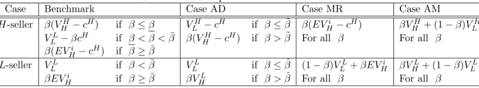
Table 1: Probabilities of trading
Benchmark Case AD Case MR Case AM
αβ+ (1 − α) if β ≤ β 1 if β ≤ ˜β αβ+ (1 − α) β
αβ+ (1 − α)[γβ + (1 − γ)] if β < β < ¯β β if β > ˜β for all β for all β
β if β ≥ ¯β β if β > ˆβ
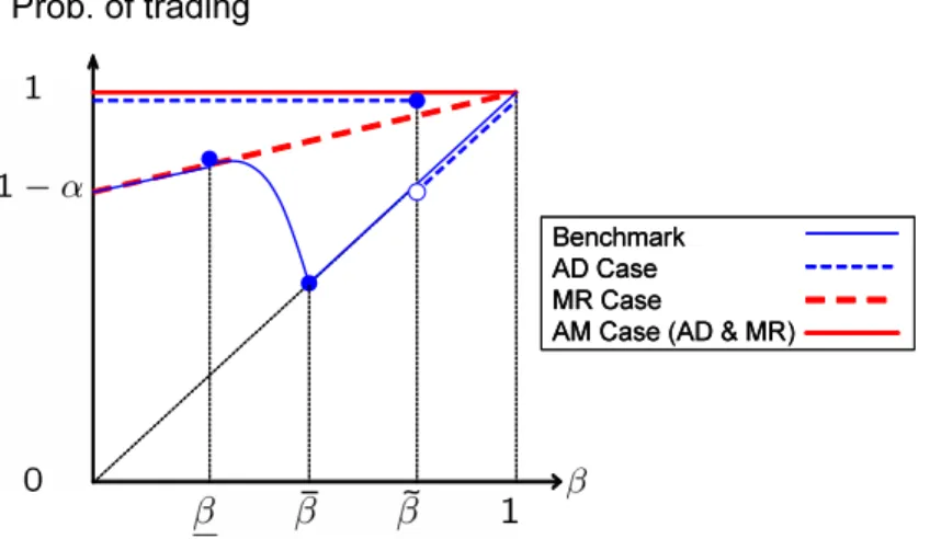
Market research First, we consider a probability of trading in each case. Since all agents have quasi-linear utility functions, any outcome is Pareto efficient if and only if the sum of the agents’ utilities is maximized. In addition, trading is always desirable, meaning that the buyer’s reservation value is always greater than the seller’s reservation value. Thus, the market efficiency can be measured by the probability of trading between the seller and the buyer. The probabilities of trading are summarized in Figure 2 and Table 1.
We consider an impact of only MR on a probability of trading by comparing the case MR with the benchmark. As shown in Figure 3, MR increases a probability of trading. Especially, for β ≥ β, MR enhances the L-seller to trade with the L-buyer, and then increases a probability of trading. For such a high value of β, if the L-seller is forced to offer a single price, then she optimally offers a high price which is acceptable to only the H-buyer in order to maximize her expected profit. In such a case, MR allows the L-buyer to discriminate prices, and then creates an additional opportunity to trade between the L-seller and the L-buyer, improving efficiency. For β ≤ β, the L-seller offers a low price and trades with the L-buyer in the benchmark, thus a probability of trading does no change in the case MR.
Next, we consider an additional valuation of MR for the seller. As noted in the previous section, the H-seller cannot increase a revenue at all by using MR in the case MR, thus an additional valuation of MR for the H-seller is zero. Furthermore, the H-seller’s expected revenue is lower in the case MR than the benchmark if β < ¯β, and is the same if β ≥ ¯β.
Unlike the H-seller, an additional valuation of MR for the L-seller is strictly positive, which is equal to the equilibrium MR fee in the case MR. Furthermore, the L-seller’s expected revenue is higher in the case MR than the benchmark for all β.
We summarize the above observation as Proposition 7.
Prob. of trading
Figure 2 Probability of trading in four cases Benchmark AD Case MR Case
AM Case (AD & MR) Benchmark AD Case MR Case
AM Case (AD & MR)
Probability one
Prob. of trading
Figure 3 Probability of trading in the case AM Probability one
Probability Probability
Proposition 7 (Market efficiency) (1) If β > β, MR creates a trade between the L-seller and the L-buyer, and increases a probability of trading as compared with the benchmark, improving market efficiency. If β ≤ β, MR has no effect on a probability of trading.
(2) The additional valuation of MR is zero for the H-seller, while strictly positive for the L-seller. The H-seller gains a lower revenue in the case MR than the benchmark, while L-seller gains a higher revenue in the case MR than the benchmark.
Advertising Before we discuss an effect of mixing AD and MR, we consider an impact of AD on a probability of trading by comparing the case AD with the benchmark. As easily can be seen in Figure 3, AD increases a probability of trading. Especially, for β ≤ ˜β, AD enhances the H-seller to trade with the L-buyer, and then increases a probability of trading. Low prices make the buyer infer than he faces the L-seller, thus the H-seller must often give up to charge low prices, leading inefficiency. In such a case, AD can make the buyer form the correct belief, and then the buyer accepts the low prices, improving efficiency.
Next, we consider an additional valuation of AD for the seller. As noted in the previous section, the L-seller cannot increase a revenue at all by using AD in the case AD, thus an additional valuation of AD for the L-seller is zero. Furthermore, the L-seller’s expected revenue is lower in the case AD than the benchmark if β > ˆβ, and is the same if β ≤ ˆβ.
Unlike the L-seller, an additional valuation of MR for the H-seller is strictly positive, which is equal to the equilibrium AD fee in the case AD. Furthermore, the H-seller’s expected revenue is higher in the case AD than the benchmark for all β.
We summarize the above observation as Proposition 8.
Proposition 8 (Advertising) (1) If β ≤ ˜β, AD creates a trade between the H-seller and the L-buyer, and increases a probability of trading as compared with the benchmark, improving market efficiency. If β > ˜β, AD has no effect on a probability of trading.
(2) The additional valuation of AD is zero for the L-seller, while strictly positive for the H-seller. The L-seller gains a lower revenue in the case AD than the benchmark, while H-seller gains a higher revenue in the case MR than the benchmark.
Synergy effect of marketing mix We consider an impact of both MR and AD on a probability of trading by comparing the case AM with the case MR, and the case AM with the case AD. As we said, if the H-seller uses AD in equilibrium and the seller’s types becomes public information, both types of sellers then prefer to use MR for sufficiently low MR fee. If, actually, both types of sellers use MR in equilibrium, then information asymmetry fully disappears, and thus the trading occurs with probability one. However, since the H-seller’s willingness to pay for MR differs from the L-seller’s willingness to pay for MR, and since the market researcher chooses the MR service fee in order to maximize her expected profit, both types of sellers do not always use MR in equilibrium. As shown in Figure 2, the trading occurs with probability one for sufficiently large α, thus both MR and AD improves market efficiency as compared with the case AD and the case MR, independent of either VLH − VLL > cH or VLH − VLL≤ cH.
If VLH − VLL≤ cH holds, for α < 1 −V
H L−cH
VLL
and β > ˜β, the H-seller gives up to use MR due to a high MR service fee, and then the trading between the H-seller and the L-buyer does not occur, resulting in a probability of trading of 1 − α(1 − β). For β > ˜β, the probability 1 − α(1 − β) in the case AM is equal to that in the case MR, and higher than that in the case AD. Therefore, both MR and AD improves market efficiency as compared with the case AD.
If VLH − VLL ≤ cH holds, however, for α < VHcH L−V
L L
and β > ˜β, the L-seller gives up to use MR due to a high MR service fee, and then the trading between the L-seller and the L-buyer does not occur, resulting in a probability of trading of 1 − (1 − α)(1 − β), which is higher than the probability of trading in the case AD. Therefore, both MR and AD do not improve market efficiency as compared with the case AD, where only AD exists. Furthermore, whether both MR and AD can improve market efficiency as compared with the case MR depends on the value of α. The probability 1 − (1 − α)(1 − β) in the case AM is higher than the probability 1 − α(1 − β) in the case AD if and only if α ≥ 0.5. Therefore, both MR and AD improve market efficiency as compared with the case AD if and only if α ≥ 0.5. Intuitively, if a probability of the seller to be H-seller is sufficiently high, the market researcher charges the MR service fee to be low enough such that both types of sellers can use MR, rather than a high MR service
fee such that only the L-seller uses MR.
Next, we consider an additional valuation of AD and MR for the seller. As previously, the additional valuation of AD is zero for the L-seller. The additional valuation of AD for the H-seller is equal to the equilibrium AD fee, and it is the same in both the case AD and the case AM.
However, the additional valuation of MR is different in the case MR and the case AM for both types of sellers. The additional valuation of MR for the H-seller is equal to mH in the followings:
(mH = β(VHH − VLH) if β ≤ ˜β mH = (1 − β)(VLH − cH) if β > ˜β.
As easily can be seen, it is positive for the H-seller in the case AM, unlike as in the case MR. Therefore, for the H-seller, there exists a positive synergy effect of marketing mix, i.e., using both AD and MR.
The additional valuation of MR for the L-seller in the case AM is equal to mLin Proposition 6, while the additional valuation of MR for the L-seller in the case MR is equal to m in Proposition 5. Comparing mL with m induces that the L-seller has the higher additional valuation of MR in the case MR than the case AM if β ≤ ˆβ, while the same additional valuation of MR in the case MR and the case AM if β > ˆβ.
We summarize the above observation as Proposition 9.
Proposition 9 (Synergy effect) (1) Both AD and MR ensure trading with probability one except the case of β > ˜β. If β > ˜β, both AD and MR achieve trading with a probability one for sufficiently high α, such as α ≥ VHcH
L −V L L
if VLH−VLL> cH, and α ≥ 1−V
H L−cH
VLL if V H
L −VLL≤ cH.
Furthermore, if VLH − VLL > cH and α < min{VHcH L −V
L L
, 0.5}, then both AD and MR worsen market efficiency as compared with the case MR.
(2) Both AD and MR increases the additional valuation of MR for the H-seller as compared with the case MR. That is, there exists a positive synergy effect of marketing mix the H-seller. However, the L-seller has the lower additional valuation of MR in the case AM than the case MR if β ≤ ˆβ, while the same in the case AM and the case MR if β > ˆβ.
Table 2: The equilibrium prices
Case Benchmark Case AD Case MR Case AM
H-seller VHH if β ≤ β VLH if β ≤ ˜β EVHi VHH and VLH
˜
p if β < β < ¯β VHH if β > ˜β for all β for all β EVHi if β ≥ ¯β
L-seller VLL if β ≤ β VLL if β ≤ ˆβ VLL and EVHi VHL and VLL VLL and ˜p if β < β < ¯β VHL if β > ˆβ for all β for all β EVHi if β ≥ ¯β
Table 3: The seller’s expected revenues
Case Benchmark Case AD Case MR Case AM
H-seller β(VHH − cH) if β ≤ β VLH − cH if β ≤ ˜β β(EVHi − cH) βVHH + (1 − β)VLH VLL− βcH if β < β < ¯β β(VHH − cH) if β > ˜β For all β For all β
β(EVHi − cH) if β ≥ ¯β
L-seller VLL if β < ¯β VLL if β ≤ ˆβ (1 − β)VLL+ βEVHi βVHL+ (1 − β)VLL βEVHi if β ≥ ¯β βVHL if β > ˆβ For all β For all β
L-seller’s
expected revenue
Figure 4 (a) Seller’s expected revenues
Benchmark AD Case MR Case
AM Case (AD & MR) Benchmark
AD Case MR Case
AM Case (AD & MR)
H-seller’s expected revenue
Figure 4 (b) Seller’s expected revenues
Benchmark AD Case MR Case
AM Case (AD & MR) Benchmark AD Case MR Case
AM Case (AD & MR)
5 Discussion
We assumed that both AD and MR can perfectly reveal seller’s and buyer’s private information. However, this assumption may not be realistic. In this section, we analyze imperfect MR and imperfect AD.
5.1 Imperfect market research
First, we consider the case in which only imperfect MR is available. We consider imperfect MR as follows: even though the seller uses MR, she only knows the buyer’s type with probability ϵ∈ [0, 1]; therefore, she still keeps the initial belief about the buyer’s type (β, 1 − β). Notice again that at least one type of the seller uses MR in a PBE. As in section 3, the H-seller does not use MR for any m ≥ 0; therefore, only the L-seller uses imperfect MR. In equilibrium, the L-seller chooses the high pooling price p∗ = EVHi to H-buyer and the lowest price pL= VLL to the L-buyer. If she cannot know the buyer’s type even though she uses MR, she chooses p∗ if β > ¯β and pL if β ≤ ¯β. We denote the i-seller’s revenue by ˆΠi[M R] and the equilibrium MR service fee by ˆm∗. The L-seller uses imperfect MR and earns revenue given by:
ΠˆL[M R] =
((1 − ϵ)[βEVHi + (1 − β)VLL] + ϵVLL= (1 − ϵ)βEVHi + (1 − β + ϵβ)VLL if β ≤ ¯β, (1 − ϵ)[βEVHi + (1 − β)VLL] + ϵEVHi = (1 + ϵ − ϵβ)EVHi + (1 − β)(1 − ϵ)VLL if β > ¯β. Notice that ˆΠL[M R] < ΠL[M R] and ˆΠL[M R] → ΠL[M R] as ϵ → 0.
The equilibrium MR service fee is given by:
ˆ m∗ =
((1 − ϵ)βEVHi − βVLL if β ≥ ¯β (1 − ϵ)(1 − β)VLL if β < ¯β.
Notice that ˆm∗ < m∗ and ˆm∗ → m∗ as ϵ → 0. Imperfect MR is less attractive for the L-seller than perfect MR. The H-seller’s strategy is the same in Proposition 4.
Next, we consider the case in which both AD and MR are available but only MR is imperfect. Since AD can perfectly reveal the quality, the H-seller uses AD in equilibrium. Again, both types of the seller use imperfect MR in equilibrium as in the previous section 3. We denote the i-seller’s revenue by ˆΠi[AM ] and the equilibrium MR service fee by ˆm∗:
ΠˆH[AM ] =
([ϵ + (1 − ϵ)(1 − β)](VLH − cH) + (1 − ϵ)β(VHH − cH) if β ≤ ˜β (1 − ϵ)(1 − β)(VLH − cH) + β(VHH − cH) if β > ˜β
ΠˆL[AM ] =
([ϵ + (1 − ϵ)(1 − β)]VLL+ (1 − ϵ)βVHL if β ≤ ˜β (1 − ϵ)(1 − β)VLL+ βVHL if β > ˜β
Notice that ˆΠH[AM ] < ΠH[AM ] and ˆΠL[AM ] < ΠL[AM ], and ˆΠH[AM ] → ΠH[AM ] and ΠˆL[AM ] → ΠL[AM ] as ϵ → 0. Furthermore, ˆΠH[AM ] → ΠH[AD] as ϵ → 1.
This comparison of revenues indicates that a synergy effect between AD and MR for the H-seller that vanishes as ϵ → 1.
The equilibrium MR fee is given by:
ˆ m∗ =
((1 − ϵ)EVHi − βVLL if β ≤ β∗ (1 − ϵ)(1 − β)VLL if β > β∗. Again ˆm∗ < m∗ and ˆm∗→ m∗ as ϵ → 0.
5.2 Imperfect advertising
We consider the case in which only AD is available. We consider imperfect AD as follows: even though the seller uses AD, if the buyer only knows the quality with probability η ∈ [0, 1], then she still keeps the initial belief about the quality (α, 1 − α). Notice that the seller cannot observe whether the buyer correctly knows the quality.
First, we consider a PBE in which only one type of seller uses imperfect AD. The buyer can perfectly distinguish the quality by the seller’s advertising behavior even though he cannot
judge the quality because of the imperfection of AD. Therefore, only the H-seller uses imperfect AD, and the same separating PBE as in the case AD is realized for any η.
Second, we consider a PBE in which both sellers use imperfect AD. Since the buyer can only distinguish the quality with probability η from the seller’s advertising behavior, the equilibrium price must be pooling: p∗ = EVLi if β is small and p∗ = EVHi if β is large. However, p∗ cannot be the equilibrium price by Assumption 2; therefore, a PBE does not exist if β is small. We denote the i-seller’s revenue by ˆΠi[AD] and the equilibrium AD service fee by ˆa∗:
( ˆΠH[AD] = β(EVHi − cH) ΠˆL[AD] = (1 − η)βEVHi. The equilibrium AD fee is given by:
ˆ
a∗ = (1 − η)βEVHi − βVLL. (6)
A PBE exists in which both types of sellers use AD if and only if both β and η are sufficiently large. This implies that the synergy effect between AD and MR for the H-seller vanishes for sufficiently large η if AD is imperfect.
6 Conclusion
We developed a model where the seller has private information about product quality while the buyer has private information about his interest in the product. The seller has two instruments potentially improving her revenue and market efficiency. Advertising can perfectly convey product quality to the buyer. Market research reveals the buyer’s type to the seller. We considered the impact of advertising and market research on market efficiency and the seller’s revenue. We obtained four major findings. First, using market research alone brings a positive benefit to the low type seller but no profit to the high type seller. Second, market research alone reduces the equilibrium price of the high type buyer, lowering the expected profit of the high type seller as well. Third, market research alone does not improve market efficiency. Fourth, the combination of advertising and market research creates a synergy, which helps the high type seller but not the low type seller. The synergy effect may explain why most firms combine advertising and market research in actual business transactions.
Three possible extensions are obvious. First, we could consider experience goods markets where informative advertising and informative market research exist. There are many kinds of experience goods for which advertising cannot convey direct information of product quality. The relation between uninformative advertising and informative market research is, however, more subtle. Furthermore, advertising has many more functions; for instance, demand stim- ulation. We could also extend the model so that advertising has several different functions. Second, we consider two marketing activities; however, there are a variety of methods that can potentially improve a seller’s profit in real business transactions. We could determine the optimal marketing mix by making other marketing methods available to the seller. Third, we assumed that the product has only two possible qualities and the buyer also has only two possible types. However, there are many types of both sellers and buyers in a real world. Thus, increasing the number of types is a natural extension. These topics will be addressed in future research.
7 References
1. Akerlof, G.A. “The Market for ‘Lemons’: Quality Uncertainty and the Market Mecha- nism.” Quarterly Journal of Economics, Vol.84 (1970), pp.488-500.
2. Allenby, G.M. and Rossi, P.E. “Marketing Models of Consumer Heterogeneity.” Journal of Econometrics, Vol.89 (1999), pp.57-78.
3. Besanko, D., Dube, J.P. and Gupta, S. “Competitive Price Discrimination Strategies in a Vertical Channel Using Aggregate Retail Data.” Management Science, Vol.49 (2003), pp.1121-1138.
4. Biglaiser, G. “Middlemen as Experts.” The RAND Journal of Economics, Vol.24 (1993), pp.212-223.
5. Biglaiser, G. and Friedman, J. “Middlemen as Guarantors of Quality.” International Journal of Industrial Organization, Vol.12 (1994), pp.509-531
6. Cabinet Office. “Annual Economic Report 1999” (in Japanese) The report can be ac- cessed at www5.cao.go.jp/j-j/wp/wp-je99/wp-je99-000i1.html