A Framework on Low Complexity Static Learning
1Emil Gizdarski
2Hideo Fujiw ara
Department of Computer Systems Nara Institute of Science and Technology University of Rousse, 7017 Rousse, Bulgaria Ikoma, Nara 630-0101, Japan
E-mail: [email protected] E-mail: [email protected]
1 This work was supported by JSPS under grant P99747
2 Currently visiting at Nara Institute of Science and Technology
ABSTRACT
In this paper, we present a new data structure for a complete implication graph and two techniques for low complexity static learning. We show that using static indirect ∧-implications and super gate extraction some hard-to-detect static and dynamic indirect implications are easily derived during static and dynamic learning as well as branch and bound search. Experimental results demonstrate the effectiveness of the proposed learning techniques.
1. INTRODUCTION
In recent years substantial progress has been achieved in Electronic Design Automation (EDA) using the Boolean satisfiability (SAT) method. The reason is development and elaboration of efficient learning techniques. Originally implemented in ATPG systems FAN[1] and SOCRATES[2], learning finds static indirect implications during preprocessing as well as dynamic implications during test generation. Further improvement of the learning techniques has been achieved in Nemesis[3] and TRAN[4] based on the Boolean satisfiability method. The first complete learning algorithm, called recursive learning, has been introduced in [5]. Now, the learning techniques are widely used in many SAT-based applications such as logic optimization, verification and test generation.
In general, learning plays a key role in avoiding unnecessary backtracking during branch and bound search by finding as many as possible implications at each level of the decision tree. Clearly, if all implications are derived during branch and bound search, each instance can be solved without backtracking. However, the deriving all implications is also an NP-complete problem. Therefore, increasing the precision of learning and keeping its complexity as low as possible is an important issue for many SAT-based applications.
The rest of this paper is organized as follows. In Sections 2 and 3, the basic learning techniques and procedures are provided. In Section 4, we present a new data structure for a complete implication graph and two new techniques for low complexity static learning. Experimental results are given in Section 5, and we conclude in Section 6.
2. BASIC LEARNING TECHNIQUES
The Boolean satisfiability method gives an elegant formulation of many EDA problems. In general, the SAT-based algorithms translate a problem to a formula that represents the constraints for the possible solutions. The formula is usually written in Conjunctive Normal Form (CNF) where one sum is called a clause. Clauses with one, two, three, or more variables are called unary, binary, ternary, and k-nary clauses respectively. The first step in satisfying a formula is to construct an implication graph. More formally, each variable X is represented by two nodes X and X . Each binary clause (X ∨ Y) is represented by two implications ( X → Y) and ( Y → X). Thus, the formula can be easily manipulated since a binding procedure requires only a partial traversal of the implication graph and checking the k- nary clauses [3]. In this way, the implication graph represents only the binary clauses. In [6], an efficient data structure representing all clauses of the CNF formula has been implemented. The resultant implication graph is called complete and contains two types of nodes. While the first type nodes represent the variables, the second type, called ∧-nodes, symbolize an conjunction operation or simply a direct ∧-implication. In the complete implication graph, each ternary clause is uniquely represented by three direct ∧-implications, see Figure 1. However, this approach requires dedicated transformation of the k-nary clauses into ternary.
The premier learning procedures [1,2] are able to find a limited set of indirect implications. Also, the precision of static learning in [2,3] strongly depends on the order of value assignments since some indirect implications can be found if certain other indirect implications have already been derived. To avoid this dependency, we assume an iterative computation of the indirect implications [7]. The iterative static learning procedure performs both 0 and 1 value assignments through the variables until one full iteration produces no new implications.
2.1. Contradiction (learning rule 1)
In [2], static learning is performed as a preprocessing phase based on the contrapositive law, (X→Y) ⇔ ( Y → X ), called here a learning rule 1. Clearly, the 2CNF portion of a formula
Figure 1: Implications for binary and ternary clauses
Permission to make digital or hard copies of all or part of this work for personal or classroom use is granted without fee provided that copies are not made or distributed for profit or commercial advantage and that copies bear this notice and the full citation on the first page. To copy otherwise, or republish, to post on servers or to redistribute to lists, requires prior specific permission and/or a fee.
DAC’01, June 18-22, 2001, Las Vegas, NV
Copyright 2000 ACM 1-58113-000-0/00/0000…$5.00.
X
Y X
Y
(X ∨ Y ∨ Z):
Y
Y X
Z Z
X ∧
∧ ∧ (X ∨ Y):
38th Design Automation Conference, Las Vegas Convention Center, pp. 546-549, June 18-22, 2001.
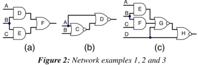
(only the binary clauses) priory fulfills the contrapositive law. This is not true when the k-nary clauses are also included. For example, it is possible that a value assignment sets k-1 variables in a k-nary clause (where k≥3) and the clause is still unsatisfied. Then a direct ∧-implication is performed and the last variable of the clause is set to a value so that the clause is satisfied. For example, value assignment B=0 for the network example 1, Figure 2(a), sets variables D and E to 0 and clause (D ∨ E ∨ F ) is still unsatisfied. Next, the binding procedure performs forward
∧-implication and sets the last variable of this clause F to 0. Thus, backward indirect implication (F=1 → B=1) is found by rule 1. Also, value assignment D=1 for the network example 2, Figure 2(b), sets variables A and C to 0, and clause (A ∨ B ∨ C) is still unsatisfied. Next, the binding procedure performs a backward ∧- implication and sets the last variable B to 1. Thus, forward indirect implication (B=0 → D=0) is found by rule 1.
2.2. Indirect ∧ ∧-implication (learning rule 2)
In [8], some indirect implications are derived as an intersection of the implications for satisfying an unjustified gate, called here a learning rule 2. The static learning procedure based on rule 2 finds indirect implication (H=1 → B=1) for the network example 3, Figure 2(c). More formally, the learning procedure iterative calculates a transitive set consisting of all direct and indirect implications derived by the transitive and contrapositive laws for each value assignment. For example, since value assignment H=1 sets variables D and G to 0, then to satisfy k-nary clause (D ∨ E ∨ F ∨ G) either variable E or F must be set to 1. However, each one of these value assignments implies that variable B must be set to 1. Since B=1 is an intersection of the transitive sets of value assignments E=1 and F=1, therefore B=1 is a necessary assignment for satisfying clause (D ∨ E ∨ F ∨ G). Thus, indirect implication (H=1 → B=1) is found. Clearly, this indirect implication cannot be found by rule 1.
2.3. Recursive learning (learning rule 3.N)
The first complete learning algorithm, recursive learning called here a learning rule 3.N, is introduced in [5]. If a level of recursion N is not restricted, then all static and dynamic implications are derived during static and dynamic learning. For example, indirect implication (C=0 → L=0) for the network example 4, Figure 3, cannot be found by rules 1 and 2 while this is possible by rule 3.1 (first level recursive learning). During iterative value assignments through the variables, the static learning procedure first finds indirect implication (E=0 → H=0)
by rule 1, since value assignment H=1 sets variable E to 1. Next, value assignment C=0 sets variables E, F and H to 0, and clause (A ∨ G ∨ H) is still unsatisfied. To satisfy this clause, either variable A or G must be set to 1, but both these assignments set variable L to 0. Therefore L=0 is a necessary assignment and indirect implications (C=0 → L=0) is found. These indirect implications cannot be found by rules 1 and 2 since neither value assignment A=1 or G=1 priory implies L=0 (L=0 is not in the transitive sets of A=1 nor G=1).
3. LEARNING PROCEDURES
In this section, we make an analysis and classification of the well-known learning procedures.
3.1. Structure based
The SOCRATES learning procedure [2] temporarily sets a variable to value 0 or 1, and checks whether the variables corresponding to gate outputs are set to non-controlling value (learning criterion). In this way, the learning procedure finds the indirect implications as a result of performing only forward ∧- implications. For example, the SOCRATES learning procedure cannot find indirect implication (B=0→D=0) for the network example 2, Figure 2(b), although value assignment D=1 sets variable B to 1 because B is not a gate output.
3.2. Clause based
In [3], an improved SAT-based static learning procedure is presented. The bounding procedure first performs all implications and then all direct ∧-implications by checking k-nary clauses. Thus, new indirect implications can be easily identified since they involve at least one direct ∧-implication (reduction of a k-nary clause to unary). In this way, Nemesis finds an indirect implication (B=0 → D=0) in the network example 2, Figure 2(b).
3.3. Implication graph based
In [4], the TRAN learning procedure derives indirect implications by finding a transitive closure of the implication graph and checking for certain properties. TRAN uses a fixation, identification and exclusion to transform the k-nary clauses to binary in order to be included into the implication graph. In fact, TRAN applies rule 3.1 restricted to the unsatisfied clauses with two unspecified variables because an analysis is made only on the implication graph. In this way, TRAN finds some hard-to-detect indirect implications, like (C=0 → L=0) and (L=1 → C=1) in the network example 4, but it fails to find some indirect implications derived by rule 2. On the other hand, the dynamical update of the implication graph and the calculation of the transitive closure make this learning procedure complicated and costly.
3.4. Set algebra based
In [8], an iterative learning procedure based on rules 2 and 3.1 is presented. For each value assignment, Simprid iterative calculates two sets, transitive and contrapositive. The transitive set of a value assignment is a list of all implications derived for this assignment. While the contrapositive set of a value assignment is a list of all implication for this assignment derived by rule 1 (contradiction). For example, if value assignment A=0 sets variable B to 1, then implication B=1 is included into the transitive set of assignment A=0 and implication A=1 is included into the contrapositive set of assignment B=0.
Table 1 presents an analysis of the precision and complexity of the well-known learning procedures. The precision is evaluated by the network examples and learning rules disused in the Figure 2: Network examples 1, 2 and 3
Figure 3: Network example 4 [8]
(a) (b)
A B C
D
(c)
D
E F A
B C
A E
C B
D
G H F
A B C D F
E G
I H
J
K L
previous section. The procedures are divided into three categories, low, average and high, according to their complexity, O(MN), O(M2N) and O(MN2) respectively, where N and M are the number of variables and the average number of the variables set by each value assignment.
Table 1: The well-known learning procedures Network examples
Learning
procedures 1 2 3 4 Precision Complexity
SOCRATES[2] + - - - < rule 1 Low
Nemesis [3] + + - - rule 1 Low
TRAN [4] + + + + < rule 3.1 High
Simprid [8] + + + + rule 3.1 Average
4. NEW LEARNING TECHNIQUES
In this section, we introduce a new data structure for the complete implication graph that facilitates the deriving and performing the indirect ∧-implications.
4.1. New data structure of implication graph
Figure 4 depicts the proposed data structure of the complete implication graph. To represent a k-nary clause, this data structure needs 2k ∧-nodes organized as a one-dimensional array and a k-bit key dynamically calculated by the binding procedure. Each bit of the k-bit key corresponds to one variable in the k-nary clause. A bit is set to 1, if the corresponding variable is specified and the k- nary clause is still unsatisfied. We also use the following conventions in this data structure: 1) we represent a gate instead of a k-nary clause. In this case, we need more sophisticated processing of (k/2-1)-input XOR gates; 2) we need one extra bit in the k-bit key to represent that a gate is justified. This is the most significant bit of the k-bit key. In this way, the k-bit key becomes a negative integer when the gate is justified; 3) the less significant bit of the k-bit key corresponds to the output of the gate. In this way, we easily identify the unjustified gates and the type of ∧- implications, forward or backward. Thus, this data structure allows a unified representation of all gates as well as both direct and indirect ∧-implications. Initially, all direct ∧-implications are included into the complete implication graph. Next, all indirect ∧- implications derived during static learning are also included into the complete implication graph.
4.2. Deriving indirect ∧ ∧-implications (rule 2+)
Example 1: Let us consider how indirect implication (H=1 → B=1) in the network example 3, Figure 2(c), can be easily found by deriving the indirect ∧-implications during static learning. First, value assignment B=0 sets variables E and F to 0 and clause (E ∨ F ∨ D ∨ G) corresponding to gate G is still unsatisfied. To
take into account this relation, the learning procedure adds indirect ∧-implication B=1 to ∧-node G=<0011>, see Figure 5. Next, value assignment H=1 sets variables D and G to 0 and clause (E ∨ F ∨ D ∨ G) corresponding to gate G is still unsatisfied. Since the k-bit key of gate G is <0011>, then all implications of ∧-node G=<0011> are valid, i.e., B=1 is a necessary assignment. Thus, this learning procedure easily finds indirect implication (H=1 → B=1). This learning technique is called here a learning rule 2+. In fact, the learning rule 2+ is equivalent to rule 2 but has lower computational complexity. In addition, rule 2+ allows some dynamic implications to be easily found during dynamic learning and branch and bound search.
4.3. Super gate extraction (learning rule A1)
A super gate of gate X can be found by performing all direct backward implications of value assignment X=A where A is a non-controlling value of the gate output X.
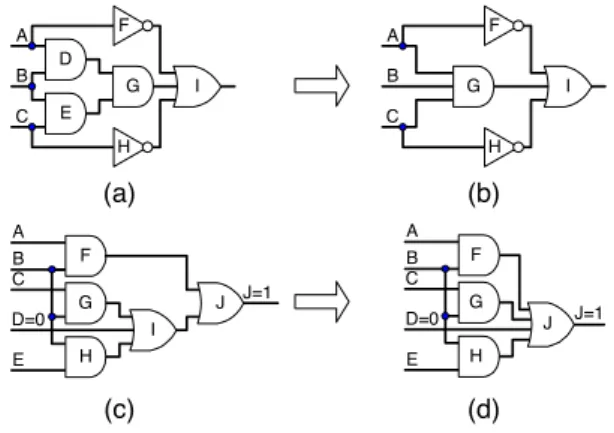
Example 2: Let us show how super gate extraction, called here an auxiliary learning rule A1, improves static learning. For the circuit shown in Figure 6(a), indirect implication (I=0 → B=0) can be found by rule 3.1 (first level recursive learning). In the transformed circuit shown in Figure 6(b), gates D, E and G are replaced by their super gate (3-input AND gate). In this case, a static indirect implication (I=0 → B=0) can be found by rule 1.
Example 3: Let us show how rule 2+ and rule A1 improve dynamic learning. After static learning based on rule 2+, two indirect ∧-implications for gate I are found for the circuit shown in Figure 6(c). After value assignment D=0, these indirect ∧- implications validate dynamic implications (I=1 → B=1) and (B=0 → I=0). Using implication (I=1 → B=1), dynamic implication (J=1→ B=1) can be found by dynamic learning based on rule 3.1 (first level recursive learning), otherwise dynamic learning based on rule 3.2 (second level recursive learning) must be applied. The dynamic implication (J=1→ B=1) can be found without dynamic learning for the transformed circuit in Figure 6(d). In this case, gates I and J form super gate J and the indirect
∧-implications of super gate J derived during static learning validate dynamic implication (J=1 → B=1) after assignment D=0.
Clearly, the proposed dada structure of the complete implication graph is not feasible for manipulation of super gates having too many inputs. To avoid a huge expansion of super gates, super gate expanding is restricted to the fanout stems. As a result, this approach decreases the number of variables, gates and stuck-at faults in the collapsed fault set of the transformed circuit. Figure 4: Representation of direct ∧-implications
Figure 5: Representation of indirect ∧-implications
Figure 6: Deriving implications using rule A1
A=0 1 1 1 1 1 0 1 0 1 1 0 0 0 1 1 0 1 0 0 0 1 0 0 0
CONFLICT
INITIALIZATION B=0
C=1
A B C (A∨B∨C) A
B C
F=1 1 1 1 1 1 1 1 0 1 1 0 1 1 1 0 0 1 0 1 1 0 1 1 1 0 0 1 1
CONFLICT
0 0 0 0 INITIALIZATION G=1 D=1
H=0 E=1 B=1 F
D (E∨F∨D∨G) G
E F D G E
C
B I
A
G F
H
C D=0 B
E A
J J=1 H
G F D
C E
B I
A
G F
H
I H G F
J C
D=0 B
E A
J=1
(a) (b)
(c) (d)
5. EXPERIMENTAL RESULTS
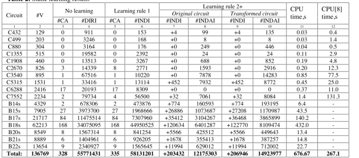
We implemented the proposed data structure and techniques in an efficient static learning procedure, and ran experiments on a 450MHz Pentium-III PC (SpecInt’95=18.7). Table 2 presents the static learning results for the ISCAS’85 and the ITC’99 benchmark circuits. Column (2) gives the number of variables (V) after super gate extraction where the size of the super gates was restricted to 13 inputs. Columns (3-6) give the number of constant assignments (CA), direct implications (DIRI) and indirect implications (INDI) before and after static learning by rule 1. As in [8], constant value assignments were not counted as implications after static learning. Also, if a value assignment sets itself and N other variables, then N+1 implications were counted. Columns (7-10) give the number of indirect implications and indirect ∧-implications (INDAI) derived by rule 2+. The contribution of rule 2, rule 2+, and rule A1 was 203432 implications, 12175303 ∧-implications, and 3514 implications and 2748674 ∧-implications respectively. Columns (11-12) give the CPU time of the proposed static learning procedure and the Simprid learning procedure [8] (based on rule 2) ran on HP 9000 J200 (SpecInt’95=4.98). After normalization, our static learning procedure is about 19 times faster than Simprid because of the new data structure of the complete implication graph that avoided the costly calculations for applying rule 2. In this experiment, we made an indirect comparison of the implications derived by our learning procedure and Simprid. The reason is that the number of variables in [8] was calculated as a sum of the number of primary inputs, primary outputs and gates. In this way, the variables corresponding to the primary outputs and the outputs of INV and EQU gates were doubled and some implications were counted twice. Also, our learning procedure further reduced the number of variables using super gate extraction. In [8], the contribution of rule 2 and rule 3.1 was 1128 and 3040 implications respectively. According to the experiment results for the ISCAS’85 benchmark circuits shown in Table 2, the contribution of rule 2 and rule 2+ was 488 implications and 35520 ∧-implications respectively. Taking into account these results, we clarify that static learning by rule 2+ is even more precise than static learning by rule 3.1 while rule 3.1 has a much higher computational complexity than rule 2+.
6. CONCLUSIONS
In this paper, we presented a new data structure of the complete implication graph and two learning techniques based on deriving and performing indirect ∧-implications and super gate extraction. The experimental results demonstrated the effectiveness of the proposed learning techniques. By keeping complexity of static learning as low as possible, we achieved a unified and fast implication procedure able to derive many hard- to-detect static and dynamic indirect implications during static learning, dynamic learning, and branch and bound search.
REFERENCES:
[1] H.Fujiwara and T.Shimono, ”On the Acceleration of Test Generation Algorithms,” IEEE Trans. on Computers, vol. C-32, No.12, December 1983, pp.1137-1144.
[2] M.Schulz, E.Trischler and T.Sarfert, "SOCRATES: A Highly Efficient Automatic Test Pattern Generation System," IEEE Trans. on CAD, vol.7, No.1, Jan. 1988, pp.126-137.
[3] T.Larrabee, "Test Pattern Generation using Boolean Satisfiability," IEEE Trans. on CAD, vol.11, No.1, Jan.1992, pp.4-15.
[4] S.Chakradhar, V.D.Agrawal and S.Rothweiler, “A Transitive Closure Algorithm for Test Generation,” IEEE Trans. on CAD, vol.12, No.7, July 1993, pp.1015-1028.
[5] W.Kunz and D.K.Pradhan, "Recursive Learning: A New Implication Technique for Efficient Solutions to CAD Problems - Test, Verification, and Optimization," IEEE Trans. on CAD, vol.13, No.9, September 1994, pp.1143-1158.
[6] P.Tafertshofer, A.Ganz and M.Henftling, "A SAT-Based Implication Engine for Efficient ATPG, Equivalence Checking, and Optimization of Netlists," Proc. IEEE ICCAD, 1997, pp.648-655. [7] P.Stephan, R.K.Brayton and A.L.Sangiovanni-Vincentelli,
”Combinational Test Generation using Satisfiability,” IEEE Trans. on CAD, vol.15, No.9, Sept. 1996, pp.1167-1176.
[8] J.Zhao, E.Rudnick and J.Patel, "Static Logic Implication with Application to Redundancy Identification," Proc. IEEE VLSI Test Symposium, 1997, pp.288-293.
Table 2: Static learning results
Learning rule 2+
No learning Learning rule 1 Original circuit Transformed circuit Circuit #V
#CA #DIRI #CA #INDI #INDI #INDAI #INDI #INDAI
CPU time,s
CPU[8] time,s
1 2 3 4 5 6 7 8 9 10 11 12
C432 129 0 911 0 153 +4 99 +4 135 0.03 0.4
C499 203 0 3246 0 168 +0 8 +0 8 0.03 1.4
C880 304 0 3164 0 176 +0 249 +0 446 0.04 0.5
C1355 515 0 19582 0 2392 +0 24 +0 24 0.11 2.9
C1908 460 0 13513 0 3267 +0 688 +0 852 0.19 4.8
C2670 826 3 14339 8 2771 +0 1593 +0 2916 0.20 12.3
C3540 895 1 67516 1 10220 +0 7878 +0 14283 0.85 77.5
C5315 1531 1 33416 1 13114 +452 7932 +452 8772 0.45 25.0
C6288 2416 17 20193 17 8309 +0 0 +0 0 0.37 11.0
C7552 2234 2 79734 4 56500 +32 7061 +32 8084 1.4 131.3
B14s 4329 2 678306 2 473876 +774 160593 +774 193195 6.4 -
B15s 7905 27 3973700 27 1968666 +26886 1073687 +27208 1170987 43.5 -
B17s 21717 84 11475514 84 7307960 +35412 3104267 +36468 3865899 140.2 -
B18s 62213 168 34075095 168 44950525 +120634 6401287 +122770 8109474 432.0 -
B20s 8549 8 1567314 8 841254 +5566 425512 +5566 449643 13.4 -
B21s 8889 6 1404961 6 926205 +1678 355413 +1678 387257 14.8 -
B22s 13654 9 2340927 9 1565645 +11994 629012 +11994 712002 22.7 -
Total: 136769 328 55771431 335 58131201 +203432 12175303 +206946 14923977 676.67 267.1