Toeplitz Inverse CovarianceBased Clustering of Multivariate Time Series Data

Toeplitz Inverse Covariance-Based Clustering of

Multivariate Time Series Data

David Hallac, Sagar Vare, Stephen Boyd, Jure Leskovec

Stanford University

{hallac,svare,boyd,jure}@stanford.edu

ABSTRACT

Subsequence clustering of multivariate time series is a useful tool for discovering repeated patterns in temporal data. Once these pat-terns have been discovered, seemingly complicated datasets can be interpreted as a temporal sequence of only a small number of states, orclusters. For example, raw sensor data from a itness-tracking application can be expressed as a timeline of a select few actions (i.e., walking, sitting, running). However, discovering these patterns is challenging because it requires simultaneous segmentation and clustering of the time series. Furthermore, interpreting the resulting clusters is diicult, especially when the data is high-dimensional. Here we propose a new method of model-based clustering, which we callToeplitz Inverse Covariance-based Clustering(TICC). Each cluster in the TICC method is deined by a correlation network, or Markov random ield (MRF), characterizing the interdependencies between diferent observations in a typical subsequence of that cluster. Based on this graphical representation, TICC simultane-ously segments and clusters the time series data. We solve the TICC problem through alternating minimization, using a variation of the expectation maximization (EM) algorithm. We derive closed-form solutions to eiciently solve the two resulting subproblems in a scalable way, through dynamic programming and the alternating direction method of multipliers (ADMM), respectively. We validate our approach by comparing TICC to several state-of-the-art base-lines in a series of synthetic experiments, and we then demonstrate on an automobile sensor dataset how TICC can be used to learn interpretable clusters in real-world scenarios.

1

INTRODUCTION

Many applications, ranging from automobiles [32] to inancial mar-kets [35] and wearable sensors [34], generate large amounts of time series data. In most cases, this data is multivariate, where each timestamped observation consists of readings from multiple enti-ties, orsensors. These long time series can often be broken down into a sequence of states, each deined by a simple łpatternž, where the states can reoccur many times. For example, raw sensor data from a itness-tracking device can be interpreted as a temporal sequence of actions [38] (i.e., walking for 10 minutes, running for

Permission to make digital or hard copies of all or part of this work for personal or classroom use is granted without fee provided that copies are not made or distributed for proit or commercial advantage and that copies bear this notice and the full citation on the irst page. Copyrights for components of this work owned by others than the author(s) must be honored. Abstracting with credit is permitted. To copy otherwise, or republish, to post on servers or to redistribute to lists, requires prior speciic permission and/or a fee. Request permissions from permissions@acm.org.

KDD ’17, August 13-17, 2017, Halifax, NS, Canada

© 2017 Copyright held by the owner/author(s). Publication rights licensed to Associa-tion for Computing Machinery.

ACM ISBN 978-1-4503-4887-4/17/08. . . $15.00 https://doi.org/10.1145/3097983.3098060

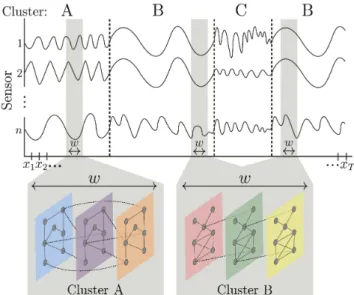
Figure 1: Our TICC method segments a time series into a se-quence of states, or łclustersž (i.e., A, B, or C). Each cluster is characterized by a correlation network, or MRF, deined over a short window of sizew. This MRF governs the (time-invariant) partial correlation structure ofany window in-side a segment belonging to that cluster. Here, TICC learns both the cluster MRFs and the time series segmentation.

30 minutes, sitting for 1 hour, then running again for 45 minutes). Similarly, using automobile sensor data, a single driving session can be expressed as a sequential timeline of a few key states: turning, speeding up, slowing down, going straight, stopping at a red light, etc. This representation can be used to discover repeated patterns, understand trends, detect anomalies and more generally, better interpret large and high-dimensional datasets.

on matching the raw values, rather than looking for more nuanced structural similarities in the data, for example how diferent sensors in a car correlate with each other across time.

In this paper, we propose a new method for multivariate time series clustering, which we callToeplitz inverse covariance-based clustering(TICC). In our method, we deine each cluster as a de-pendency network showing the relationships between the diferent sensors in a short (time-invariant) subsequence (Figure 1). For ex-ample, in a cluster corresponding to a łturnž in an automobile, this network, known as a Markov random ield (MRF), might show how the brake pedal at a generic timetmight afect the steering wheel angle at timet+1. Here, the MRF of a diferent cluster, such as łslowing downž, will have a very diferent dependency structure between these two sensors. In these MRFs, an edge represents a partial correlation between two variables [26, 41, 46]. It is impor-tant to note that MRFs denote a relationship much stronger than a simple correlation; partial correlations are used to control for the efect of other confounding variables, so the existence of an edge in an MRF implies that there is adirectdependency between two variables in the data. Therefore, an MRF provides interpretable insights as to precisely what the key factors and relationships are that characterize each cluster.

In our TICC method, we learn each cluster’s MRF by estimating a sparse Gaussian inverse covariance matrix [14, 48]. With an inverse covarianceΘ, ifΘi,j = 0, then by deinition, elementsi andj

inΘare conditionally independent (given the values of all other variables). Therefore,Θdeines the adjacency matrix of the MRF dependency network [1, 45]. This network has multiple layers, with edges both within a layer and across diferent layers. Here, the number of layers corresponds to the window size of a short subsequence that we deine our MRF over. For example, the MRFs corresponding to clusters A and B in Figure 1 both have three layers. This multilayer network represents the time-invariant correlation structure ofanywindow of observations inside a segment belonging to that cluster. We learn this structure for each cluster by solving a constrained inverse covariance estimation problem, which we call theToeplitz graphical lasso. The constraint we impose ensures that the resulting multilayer network has a block Toeplitz structure [16] (i.e., any edge between layerslandl+1 also exists between layers l+1 andl+2). This Toeplitz constraint ensures that our cluster deinitions are time-invariant, so the clustering assignment does not depend on the exact starting position of the subsequence. Instead, we cluster this short subsequence based solely on the structural state that the time series is currently in.

To solve the TICC problem, we use an expectation maximization (EM)-like approach, based on alternating minimization, where we iteratively cluster the data and then update the cluster parameters. Even though TICC involves solving a highly non-convex maximum likelihood problem, our method is able to ind a (locally) optimal solution very eiciently in practice. When assigning the data to clus-ters, we have an additional goal oftemporal consistency, the idea that adjacent data in the time series is encouraged to belong to the same cluster. However, this yields a combinatorial optimization prob-lem. We develop a scalable solution using dynamic programming, which allows us to eiciently learn the optimal assignments (it takes justO(KT)time to assign theT points intoKclusters). Then, to

solve for the cluster parameters, we develop an algorithm to solve the Toeplitz graphical lasso problem. Since learning this graphical structure from data is a computationally expensive semideinite programming problem [6, 22], we develop a specialized message-passing algorithm based on the alternating direction method of multipliers (ADMM) [5]. In our Toeplitz graphical lasso algorithm, we derive closed-form updates for each of the ADMM subproblems to signiicantly speed up the solution time.

We then implement our TICC method and apply it to both real and synthetic datasets. We start by evaluating performance on several synthetic examples, where there are known ground truth clusters. We compare TICC with several state-of-the-art time series clustering methods, outperforming them all by at least 41% in terms of cluster assignment accuracy. We also quantify the amount of data needed for accurate cluster recovery for each method, and we see that TICC requires 3x fewer observations than the next best method to achieve similar performance. Additionally, we discover that our approach is able to accurately reconstruct the underlying MRF dependency network, with anF1network recovery score between 0.79 and 0.90 in our experiments. We then analyze an automobile sensor dataset to see an example of how TICC can be used to learn interpretable insights from real-world data. Applying our method, we discover that the automobile dataset has ive true clusters, each corresponding to a łstatež that cars are frequently in. We then validate our results by examining the latitude/longitude locations of the driving session, along with the resulting clustering assignments, to show how TICC can be a useful tool for unsupervised learning from multivariate time series.

2

PROBLEM SETUP

Consider a time series ofTsequential observations,

xorig=    

| | | |

x1 x2 x3 . . . xT

| | | |

   

,

wherexi ∈Rnis thei-th multivariate observation. Our goal is to

cluster theseTobservations intoKclusters. However, instead of clustering each observation in isolation, we treat each point in the context of its predecessors in the time series. Thus, rather than just looking atxt, we instead cluster a short subsequence of sizew ≪T

that ends att. This consists of observationsxt−w+1, . . . ,xt, which

we concatenate into annw-dimensional vector that we callXt. We

refer to this new sequence, fromX1toXT, asX. Note that there is

a bijection, or a bidirectional one-to-one mapping, between each pointxtand its resulting subsequenceXt. (The irstwobservations

ofxorigsimply map to a shorter subsequence, since the time series does not start untilx1.) These subsequences are a useful tool to provide proper context for each of theTobservations. For example, in automobiles, a single observation may show the current state of the car (i.e., driving straight at 15mph), but a short window, even one that lasts just a fraction of a second, allows for a more com-plete understanding of the data (i.e., whether the car is speeding up or slowing down). As such, rather than clustering the obser-vations directly, our approach instead consists of clustering these subsequencesX1, . . . ,XT. We do so in such a way that encourages

adjacent subsequences to belong to the same cluster, a goal that we calltemporal consistency. Thus, our method can be viewed as a form of time point clustering [49], where we simultaneously segment and cluster the time series.

Toeplitz Inverse Covariance-Based Clustering (TICC).We de-ine each cluster by a Gaussian inverse covarianceΘi ∈Rnw×nw.

Recall that inverse covariances show the conditional independency structure between the variables [26], soΘi deines a Markov

ran-dom ield encoding the structural representation of clusteri. In addi-tion to providing interpretable results, sparse graphical representa-tions are a useful way to prevent overitting [27]. As such, our objec-tive is to solve for theseKinverse covariancesΘ₌{Θ₁, . . . ,ΘK},

one per cluster, and the resulting assignment setsP₌{P1, . . . ,PK},

wherePi ⊂ {1,2, . . . ,T}. Here, each of theT points are assigned to

exactly one cluster. Our overall optimization problem is

argmin

Θ∈ T,P

K X

i=1   

sparsity

z }| {

∥λ◦Θi∥1+

X

Xt∈Pi *. .. ,

log likelihood

z }| {

−ℓℓ(Xt,Θi)+

temporal consistency

z }| {

β1{Xt−1<Pi} +///

-  . (1)

We call this theToeplitz inverse covariance-based clustering(TICC) problem. Here,T is the set of symmetric block Toeplitznw×nw matrices and∥λ◦Θi∥1is anℓ1-norm penalty of the Hadamard (element-wise) product to incentivize a sparse inverse covariance (whereλ∈Rnw×nwis a regularization parameter). Additionally,

ℓℓ(Xt,Θi)is the log likelihood thatXt came from clusteri,

ℓℓ(Xt,Θi)=−1

2(Xt−µi)

T_Θ

i(Xt−µi)

+1₂log detΘi−n

2log(2π), (2)

whereµiis the empirical mean of clusteri. In Problem (1),βis a

parameter that enforces temporal consistency, and1{Xt−1<Pi}

is an indicator function checking whether neighboring points are assigned to the same cluster.

Toeplitz Matrices.Note that we constrain theΘi’s, the inverse

covariances, to be block Toeplitz. Thus, eachnw×nwmatrix can be expressed in the following form,

Θi =           

A(0) (A(1))T (A(2))T · · · (A(w−1))T

A(1) A(0) (A(1))T . .. ...

A(2) A(1) . .. . .. . .. ... .

.

. . .. . .. . .. (A(1))T (A(2))T

. .

. . .. _A(1) _A(0) _(A(1)₎T

A(w−1) · · · A(2) A(1) A(0)           

,

whereA(0),A(1), . . . ,A(w−1) ∈Rn×n. Here, theA(0)sub-block rep-resents the intra-time partial correlations, soA(0)_{i j} refers to the relationship between concurrent values of sensorsiandj. In the MRF corresponding to this cluster,A(0)deines the adjacency matrix of the edges within each layer. On the other hand, the of-diagonal sub-blocks refer to łcross-timež edges. For example,A(1)_{i j} shows how sensoriat some timetis correlated to sensorjat timet+1, and A(2)shows the edge structure between timetand timet+2. The block Toeplitz structure of the inverse covariance means that we are making a time-invariance assumption over this length-wwindow (we typically expect this window size to be much smaller than the average segment length). As a result, in Figure 1, for example, the edges between layer 1 and layer 2 must also exist between layers 2 and 3. We use this assumption because we are looking for a unique structural pattern to identify each cluster. We consider each cluster to be a certain łstatež. When the time series is in this state, it retains a certain (time-invariant) structure that persists throughout this segment, regardless of the window’s starting point. By enforcing a Toeplitz structure on the inverse covariance, we are able to model this time invariance and incorporate it into our estimate ofΘi.

Regularization Parameters.Our TICC optimization problem has two regularization parameters:λ, which determines the sparsity level in the MRFs characterizing each cluster, andβ, the smoothness penalty that encourages adjacent subsequences to be assigned to the same cluster. Note that even thoughλis anw×nwmatrix, we typically set all its values to a single constant, reducing the search space to just one parameter. In applications where there is prior knowledge as to the proper sparsity or temporal consistency,λand βcan be chosen by hand. More generally, the parameter values can also be selected by a more principled method, such as Bayesian information criterion (BIC) [18] or cross-validation.

Window Size.Recall that instead of clustering each pointxt in

isolation, we cluster a short window, or subsequence, going from timet−w+1 tot, which we concatenate into anw-dimensional vector that we callXt. The Toeplitz constraint assumes that each

larger the window, the farther these cross-time edges can reach. However, we do not want our window to be too large, since it may struggle to properly classify points at the segment boundaries, where our time-invariant assumption may not hold. For this reason, we generally keep the value ofwrelatively small. However, its exact value should generally be chosen depending on the application, the granularity of the observations, and the average expected segment length. It can also be selected via BIC or cross-validation, though as we discover in Section 6, our TICC algorithm is relatively robust to the selection of this window size parameter.

Selecting the Number of Clusters.As with many clustering al-gorithms, the number of clustersKis an important parameter in TICC. There are various methods for doing so. If there is some la-beled ground truth data, we can use cross-validation on a test set or normalized mutual information [8] to evaluate performance. If we do not have such data, we can use BIC or the silhouette score [40] to select this parameter. However, the exact number of clusters will often depend on the application itself, especially since we are also looking for interpretability in addition to accuracy.

3

ALTERNATING MINIMIZATION

Problem (1) is a mixed combinatorial and continuous optimization problem. There are two sets of variables, the cluster assignmentsP and inverse covariancesΘ, both of which are coupled together to make the problem highly non-convex. As such, there is no tractable way to solve for the globally optimal solution. Instead, we use a variation of the expectation maximization (EM) algorithm to alternate between assigning points to clusters and then updating the cluster parameters. While this approach does not necessarily reach the global optimum, similar types of methods have been shown to perform well on related problems [13]. Here, we deine the subproblems that comprise the two steps of our method. Then, in Section 4, we derive fast algorithms to solve both subproblems and formally describe our overall algorithm to solve the TICC problem.

3.1

Assigning Points to Clusters

We assign points to clusters by ixing the value ofΘand solv-ing the followsolv-ing combinatorial optimization problem forP ₌

{P1, . . . ,PK},

minimize

K X

i=1 X

Xt∈Pi

−ℓℓ(Xt,Θi)+β1{Xt−1<Pi}. (3)

This problem assigns each of theT subsequences to one of theK clusters to jointly maximize the log likelihood and the temporal consistency, with the tradeof between the two objectives regulated by the regularization parameterβ. Whenβ =0, the subsequences X1, . . . ,XT can all be assigned independently, since there is no

penalty to encourage neighboring subsequences to belong to the same cluster. This can be solved by simply assigning each point to the cluster that maximizes its likelihood. Asβgets larger, neighbor-ing subsequences are more and more likely to be assigned to the same cluster. Asβ → ∞, the switching penalty becomes so large that all the points in the time series are grouped together into just one cluster. Even though Problem (3) is combinatorial, we will see

in Section 4.1 that we can use dynamic programming to eiciently ind the globally optimal solution for this TICC subproblem.

3.2

Toeplitz Graphical Lasso

Given the point assignmentsP, our next task is to update the cluster parametersΘ₁, . . . ,ΘK by solving Problem (1) while holdingP

constant. We can solve for eachΘi in parallel. To do so, we notice

that we can rewrite the negative log likelihood in Problem (2) in terms of eachΘi. This likelihood can be expressed as

X

Xt∈Pi

−ℓℓ(Xt,Θi)=−|Pi|(log detΘi+tr(SiΘi))+C,

where|Pi|is the number of points assigned to clusteri,Si is the

empirical covariance of these points, andCis a constant that does not depend onΘi. Therefore, the M-step of our EM algorithm is

minimize −log detΘi+tr(SiΘi)+_|P1

i|

∥λ◦Θi∥1

subject to Θi ∈ T. (4)

Problem (4) is a convex optimization problem, which we call the

Toeplitz graphical lasso. This is a variation on the well-known graph-ical lasso problem [14] where we add a block Toeplitz constraint on the inverse covariance. The original graphical lasso deines a tradeof between two objectives, regulated by the parameterλ: min-imizing the negative log likelihood, and making sureΘiis sparse.

WhenSi is invertible, the likelihood term encouragesΘito be near

S_i−1. Our problem adds the additional constraint thatΘi is block

Toeplitz.λis anw×nwmatrix, so it can be used to regularize each sub-block ofΘidiferently. Note that |P1i| can be incorporated into the regularization by simply scalingλ; as such, we typically write Problem (4) without this term (and scaleλaccordingly) for notational simplicity.

4

TICC ALGORITHM

Here, we describe our algorithm to clusterX1, . . . ,XT intoK

clus-ters. Our method, described in full in Section 4.3, depends on two key subroutines: AssignPointsToClusters, where we use a dynamic programming algorithm to assign eachXtinto a cluster, and

Up-dateClusterParameters, where we update the cluster parameters by solving the Toeplitz graphical lasso problem using an algorithm based on the alternating direction method of multipliers (ADMM). Note that this is similar to expectation maximization (EM), with the two subroutines corresponding to the E and M steps, respectively.

4.1

Cluster Assignment

Given the model parameters (i.e., inverse covariances) for each of theKclusters, solving Problem (3) assigns theT subsequences, X1, . . . ,XT, to theseKclusters in such a way that maximizes the

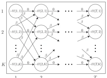
Figure 2: Problem(3)is equivalent to inding the minimum-cost path from timestamp 1 toT, where the node cost is the negative log likelihood of that point being assigned to a given cluster, and the edge cost isβ whenever the cluster assignment switches.

Algorithm 1Assign Points to Clusters

1: givenβ>0,−ℓℓ(i,j)= negative log likelihood of pointiwhen it is assigned to clusterj.

2: initializePrevCost = list ofKzeros. 3: CurrCost = list ofKzeros. 4: PrevPath = list ofKempty lists.

5: CurrPath = list ofKempty lists. 6: fori=1, . . . ,Tdo

7: forj=1, . . . ,Kdo

8: MinIndex = index of minimum value of PrevCost.

9: ifPrevCost[MinIndex] +β >PrevCost[j]then

10: CurrCost[j] = PrevCost[j]−ℓℓ(i,j). 11: CurrPath[j] = PrevPath[j].append[j].

12: else

13: CurrCost[j] = PrevCost[minIndex] +β−ℓℓ(i,j). 14: CurrPath[j] = PrevPath[minIndex].append[j].

15: PrevCost = CurrCost.

16: PrevPath = CurrPath.

17: FinalMinIndex = index of minimum value of CurrCost. 18: FinalPath = CurrPath[FinalMinIndex].

19: returnFinalPath.

4.2

Solving the Toeplitz Graphical Lasso

Once we have the clustering assignments, the M-step of our EM algorithm is to update the inverse covariances, given the points assigned to each cluster. Here, we are solving the Toeplitz graphical lasso, which is deined in Problem (4). For smaller covariances, this semideinite programming problem can be solved using standard interior point methods [6, 36]. However, to solve the overall TICC problem, we need to solve a separate Toeplitz graphical lasso for each cluster at every iteration of our algorithm. Therefore, since we may need to solve Problem (4) hundreds of times before TICC converges, it is necessary to develop a fast method for solving it

eiciently. We do so through the alternating direction method of multipliers (ADMM), a distributed convex optimization approach that has been shown to perform well at large-scale optimization tasks [5, 37]. With ADMM, we split the problem up into two sub-problems and use a message passing algorithm to iteratively con-verge to the globally optimal solution. ADMM is especially scalable when closed-form solutions can be found for the ADMM subprob-lems, which we are able to derive for the Toeplitz graphical lasso.

To put Problem (4) in ADMM-friendly form, we introduce a consensus variableZ and rewrite Problem (4) as its equivalent problem,

minimize −log detΘ+tr(SΘ)+∥λ◦Z∥₁ subject to Θ₌Z,Z∈ T.

The augmented Lagrangian [19] can then be expressed as

L_ρ(Θ,Z,U):=−log det(Θ)+Tr(SΘ)+∥λ◦Z∥1

+ρ₂∥Θ−Z+U∥2_F. (5)

whereρ>0 is the ADMM penalty parameter,U∈Rnw×nw_{is the}

scaled dual variable [5, ğ3.1.1], andZ∈ T.

ADMM consists of the following three steps repeated until con-vergence,

(a) Θk+1_:

=argmin Θ

L_ρΘ,Zk,Uk

(b) Zk+1_:

=argmin

Z∈ T

L_ρΘk+1_,Z,Uk

(c) Uk+1_:

=Uk+(Θk+1−Zk+1_),

wherek is the iteration number. Here, we alternate optimizing Problem (5) overΘand then overZ, and after each iteration we update the scaled dual variableU. Since the Toeplitz graphical lasso problem is convex, ADMM is guaranteed to converge to the global optimum. We use a stopping criteria based on the primal and dual residual values being close to zero; see [5].

Θ-Update.TheΘ-update can be written as

Θk+1

=argmin Θ

−log det(Θ)₊Tr(SΘ)₊ρ

2Θ−Z

k

+Uk2_F.

This optimization problem has a known analytical solution [10],

Θk+1

= ρ₂QD+

q

D2+4ρIQT, (6)

whereQDQT is the eigendecomposition ofZk−_ρUk −S.

Z-Update.TheZ-update can be written as

Zk+1

=argmin

Z∈ T

∥λ◦Z∥₁₊ρ 2Z−Θ

k+1_−Uk

2F. (7)

This proximal operator can be solved in parallel for each sub-block A(0),A(1), . . . ,A(w−1). Furthermore, within each sub-block, each

(i,j)-th element in the sub-block can be solved in parallel as well. In A(0), there aren(n+1)

Algorithm 2Toeplitz Inverse Covariance-Based Clustering

1: initializeCluster parametersΘ; cluster assignmentsP. 2: repeat

3: E-step:Assign points to clusters →P. 4: M-step:Update cluster parameters→Θ_.

5: untilStationarity.

return(Θ,P).

We denote the number of times each element appears asR(this equals 2(w−m)for sub-blockA(m), except for the diagonals ofA(0), which occurwtimes.) We order theseRoccurrences, and we let B_{i j}(m)

,l

refer to the index inZcorresponding to thel-th occurrence of

the(i,j)-th element ofA(m), wherel=1, . . . ,R. Thus,B(_{i j}m)

,l

returns an index(x,y)in thenw×nwmatrix ofZ. With this notation, we can solve each of the(w−1)n2+n(n₂+1) subproblems of theZ -update proximal operator the same way. To solve for the elements ofZcorresponding toB_{i j}(m), we set these elements all equal to

argmin

z R X

l=1

|λ_B(m)

i j,l

z|₊ρ 2 z−(Θ

k+1

+Uk)_B(m)

i j,l

!2

. (8)

We letQ =PR_l=1λ_B(m)

i j,l

andSl =(Θk+1_+Uk₎ B_{i j}(m)

,l

for notational

simplicity. Then, Problem (8) can be rewritten as

argmin

z Q

|z|₊

R X

l=1

ρ 2(z−Sl)

2_.

This is just a soft-threshold proximal operator [37], which has the following closed-form solution,

Zk+1

Bi j(m) =

 

ρPlSl−Q

ρR

ρPlSl−Q

ρR >0

ρPlSl+Q ρR

ρPlSl+Q

ρR <0

0 otherwise.

(9)

We ill in theRelements inZk+1_{(corresponding toB}(m)

i j ) with this

value. We do the same for all(w−1)n2+n(n₂+1) subproblems, each of which we can solve in parallel, and we are left with our inal result for the overallZ-update.

4.3

TICC Clustering Algorithm

To solve the TICC problem, we combine the dynamic programming algorithm from Section 4.1 and the ADMM method in Section 4.2 into one iterative EM algorithm. We start by randomly initializing the clusters. From there, we alternate the E and M-steps until the cluster assignments are stationary (i.e., the problem has converged). The overall TICC method is outlined in Algorithm (2)

5

IMPLEMENTATION

We have built a custom Python solver to run the TICC algorithm1. Our solver takes as inputs the original multivariate time series and the problem parameters. It then returns the clustering assignments of each point in the time series, along with the structural MRF representation of each cluster.

1_{Code and solver are available at http://snap.stanford.edu/ticc/.}

6

EXPERIMENTS

We test our TICC method on several synthetic examples. We do so because there are known łground truthž clusters to evaluate the accuracy of our method.

Generating the Datasets.We randomly generate synthetic multi-variate data inR5. Each of theKclusters has a mean of⃗0 so that the clustering result is based entirely on the structure of the data. For each cluster, we generate a random ground truth Toeplitz inverse covariance as follows [33]:

(1) SetA(0),A(1), . . .A(4) ∈R5×5equal to the adjacency matrices of 5 independent Erdős-Rényi directed random graphs, where every edge has a 20% chance of being selected.

(2) For every selected edge inA(m)setA_jk(m) =vjk,m, a random

weight centered at 0 (For theA(0) block, we also enforce a symmetry constraint that everyA(0)_{i j} =A(0)ji ).

(3) Construct a 5w×5wblock Toeplitz matrixG, wherew=5 is the window size, using the blocksA(0),A(1), . . .A(4).

(4) Letcbe the smallest eigenvalue ofG, and setΘi =G+(0.1+|c|)I. This diagonal term ensures thatΘi is invertible.

The overall time series is then generated by constructing a temporal sequence of cluster segments (for example, the sequence ł1,2,1ž with 200 samples in each of the three segments, coming from two inverse covariancesΘ₁andΘ₂). The data is then drawn one sample at a time, conditioned on the values of the previousw−1 samples. Note that, when we have just switched to a new cluster, we are drawing a new sample in part based on data that was generated by the previous cluster.

We run our experiments on four diferent temporal sequences: ł1,2,1ž, ł1,2,3,2,1ž, ł1,2,3,4,1,2,3,4ž, ł1,2,2,1,3,3,3,1ž. Each segment in each of the examples has 100Kobservations inR5, whereKis the number of clusters in that experiment (2, 3, 4, and 3, respectively). These examples were selected to convey various types of temporal sequences over various lengths of time.

Performance Metrics.We evaluate performance by clustering each point in the time series and comparing to the ground truth clusters. Since both TICC and the baseline approaches use very similar methods for selecting the appropriate number of clusters, we ixKto be the łtruež number of clusters, for both TICC and for all the baselines. This yields a straightforward multiclass classii-cation problem, which allows us to evaluate clustering accuracy by measuring the macro-F1score. For each cluster, theF1score is the harmonic mean of the precision and recall of our estimate. Then, the macro-F1score is the average of theF1scores for all the clusters. We use this score to compare our TICC method with several well-known time series clustering baselines.

Baseline Methods.We use multiple model and distance-based clustering approaches as our baselines. The methods we use are:

• TICC,β =0 Ð This is our TICC method without the temporal consistency constraint. Here, each subsequence is assigned to a cluster independently of its location in the time series. • GMM Ð Clustering using a Gaussian Mixture Model [2]. • EEV Ð Regularized GMM with shape and volume constraints

Temporal Sequence

Clustering Method 1,2,1 1,2,3,2,1 1,2,3,4,1,2,3,4 1,2,2,1,3,3,3,1

TICC 0.92 0.90 0.98 0.98

Model-TICC,β=0 0.88 0.89 0.86 0.89

Based

GMM 0.68 0.55 0.83 0.62

EEV 0.59 0.66 0.37 0.88

Distance-DTW, GAK 0.64 0.33 0.26 0.27

Based

DTW, Euclidean 0.50 0.24 0.17 0.25

Neural Gas 0.52 0.35 0.27 0.34

K-means 0.59 0.34 0.24 0.34

Table 1: Macro-F1score of clustering accuracy for four dif-ferent temporal sequences, comparing TICC with several al-ternative model and distance-based methods.

100 200 300 400 500

Number of Samples per Segment

0.0

0.2

0

.4

0

.6

0

.8

1

.0

M

a

c

ro

-F

1

S

c

o

re

TICC TICC, B=0

GMM EEV

DTW, GAK DTW, Euclidean

Neural Gas K-means

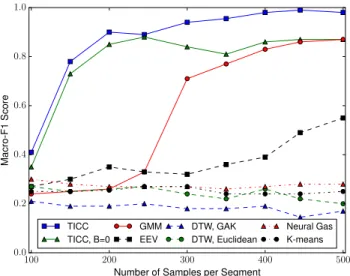
Figure 3: Plot of clustering accuracy macro-F1score vs. num-ber of samples for TICC and several baselines. TICC needs signiicantly fewer samples than the other model-based methods to achieve similar performance, while the distance-based measures are unable to capture the true structure.

•DTW, GAK Ð Dynamic time warping (DTW)-based clustering using a global alignment kernel [9, 42].

•DTW, Euclidean Ð DTW using a Euclidean distance metric [42]. •Neural Gas Ð Artiicial neural network clustering method,

based on self-organizing maps [12, 31].

•K-means Ð The standard K-means clustering algorithm using Euclidean distance.

Clustering Accuracy.We measure the macro-F1score for the four diferent temporal sequences in Table 1. Here, all eight methods are using the exact same synthetic data, to isolate each approach’s efect on performance. As shown, TICC signiicantly outperforms the baselines. Our method achieves a macro-F1score between 0.90 and 0.98, averaging 0.95 across the four examples. This is 41% higher than the second best method (not counting TICC,β =0), which is GMM and has an average macro-F1score of only 0.67. We also ran our experiments using micro-F1score, which uses a weighted average to weigh clusters with more samples more heavily, and we obtained very similar results (within 1-2% of the macro-F1scores). Note that theKclusters in our examples are always zero-mean, and that they are only diferentiated by the structure of the data. As a result, the distance-based methods struggle at identifying the

Temporal Sequence TICC Network RecoveryF1score

1,2,1 0.83

1,2,3,2,1 0.79

1,2,3,4,1,2,3,4 0.89 1,2,2,1,3,3,3,1 0.90

Table 2: Network edge recoveryF1score for the four tempo-ral sequences. TICC deines each cluster as an MRF graphi-cal model, which is successfully able to estimate the depen-dency structure of the underlying data.

clusters, and these approaches have lower scores than the model-based methods for these experiments.

Efect of the Total Number of Samples.We next focus on how many samples are required for each method to accurately cluster the time series. We take the ł1,2,3,4,1,2,3,4ž example from Table 1 and vary the number of samples. We plot the macro-F1score vs. number of samples per segment for each of the eight methods in Figure 3. As shown, when there are 100 samples, none of the methods are able to accurately cluster the data. However, as we observe more samples, both TICC and TICC,β=0 improve rapidly. By the time there are 200 samples, TICC already has a macro-F1 score above 0.9. Even when there is a limited amount of data, our TICC method is still able to accurately cluster the data. Additionally, we note that the temporal consistency constraint, deined byβ, has only a small efect in this region, since both TICC and TICC, β =0 achieve similar results. Therefore, the accurate results are most likely due to the sparse block Toeplitz constraint that we impose in our TICC method. However, as the number of samples increases, these two plots begin to diverge, as TICC goes to 1.0 while TICC,β =0 hovers around 0.9. This implies that, once we have enough samples, the inal improvement in performance is due to the temporal consistency penalty that encourages neighboring samples to be assigned to the same cluster.

Network Recovery Accuracy.Recall that our TICC method has the added beneit in that the clusters it learns are interpretable. TICC models each cluster as a multilayer Markov random ield, a network with edges corresponding to the non-zero entries in the inverse covariance matrixΘi. We can compare our estimated

network with the łtruež MRF network and measure the average macro-F1score of our estimate across all the clusters. We look at the same four examples as in Table 2 and plot the results in Table 2. We recover the underlying edge structure of the network with anF1 score between 0.79 and 0.90. This shows that TICC is able to both accurately cluster the data and recover the network structure of the underlying clusters. Note that our method is the irst approach that is able to explicitly reconstruct this network, something that the other baseline methods are unable to do.

104 ₁₀5 ₁₀6 ₁₀7 Number of Observations

101

102

103

104

T

IC

C

R

u

n

ti

m

e

(S

e

c

o

n

d

s

)

Figure 4: Per-iteration runtime of the TICC algorithm (both the ADMM and dynamic programming steps). Our algo-rithm scales linearly with the number of samples. In this case, each observation is a vector in R50.

other three examples, so our TICC method appears to be relatively robust to the selection ofw.

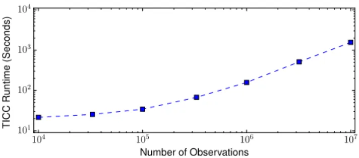
Scalability of TICC.One iteration of the TICC algorithm consists of running the dynamic programming algorithm and then solving the Toeplitz graphical lasso problem for each cluster. These steps are repeated until convergence. The total number of iterations depends on the data, but typically is no more than a few tens of iterations. SinceT is typically much larger than bothKandn, we can expect the largest bottleneck to occur during the assignment phase, whereT can potentially be in the millions. To evaluate the scalability of our algorithm, we varyTand compute the runtime of the algorithm over one iteration. We observe samples inR50, estimate 5 clusters with a window size of 3, and varyT over several orders of magnitude. We plot the results in log-log scale in Figure 4. Note that our ADMM solver infers each 150×150 inverse covariance (sincenw =50×3=150) in under 4 seconds, but this runtime is independent ofT, so ADMM contributes to the constant ofset in the plot. As shown, at large values ofT, our algorithm scales linearly with the number of points. Our TICC solver can cluster 10 millions points, each inR50, with a per-iteration runtime of approximately 25 minutes.

7

CASE STUDY

Here, we apply our TICC method to a real-world example to demon-strate how this approach can be used to ind meaningful insights from time series data in an unsupervised way.

We analyze a dataset, provided by a large automobile company, containing sensor data from a real driving session. This session lasts for exactly 1 hour and occurs on real roads in the suburbs of a large European city. We observe 7 sensors every 0.1 seconds:

•Brake Pedal Position •Forward (X-)Acceleration •Lateral (Y-)Acceleration •Steering Wheel Angle

• Vehicle Velocity • Engine RPM • Gas Pedal Position

Thus, in this one-hour session, we have 36,000 observations of a 7-dimensional time series. We apply TICC with a window size of 1 second (or 10 samples). We pick the number of clusters using BIC, and we discover that this score is optimized atK=5.

We analyze the 5 clusters outputted by TICC to understand and interpret what łdriving statež they each refer to. Each cluster has a multilayer MRF network deining its structure. To analyze the result, we use network analytics to determine the relative łimportancež

Interpretation Brake X-Acc Y-Acc SW Angle Vel RPM Gas

#1 Slowing Down 25.64 0 0 0 27.16 0 0

#2 Turning 0 4.24 66.01 17.56 0 5.13 135.1

#3 Speeding Up 0 0 0 0 16.00 0 4.50

#4 Driving Straight 0 0 0 0 32.2 0 26.8

#5 Curvy Road 4.52 0 4.81 0 0 0 94.8

Table 3: Betweenness centrality for each sensor in each of the ive clusters. This score can be used as a proxy to show how łimportantž each sensor is, and more speciically how much it directly afects the other sensor values.

of each node in the cluster’s network. We plot the betweenness centrality score [7] of each node in Table 3. We see that each of the 5 clusters has a unique łsignaturež, and that diferent sensors have diferent betweenness scores in each cluster. For example, the Y-Acceleration sensor has a non-zero score in only two of the ive clusters: #2 and #5. As such, we would expect these two clus-ters to refer to states in which the car is turning, and the other three clusters to refer to intervals where the car is going straight. Similarly, cluster #1 is the only cluster with no importance on the Gas Pedal, and it is also the cluster with the largest Brake Pedal score. Therefore, we expect this state to be the cluster assignment whenever the car is slowing down. We also see that clusters 3 and 4 have the same non-zero sensors, velocity and gas pedal, so we may expect them to refer to states when the car is driving straight and not slowing down, with the most łimportantž sensor in the two clusters being the velocity in cluster 4. As such, we can use these betweenness scores to interpret these clusters in a meaningful way. For example, from Table 3, a reasonable hypothesis might be that the clusters refer to 1) slowing down, 2) turning, 3) speeding up, 4) cruising on a straight road, 5) driving on a curvy road segment.

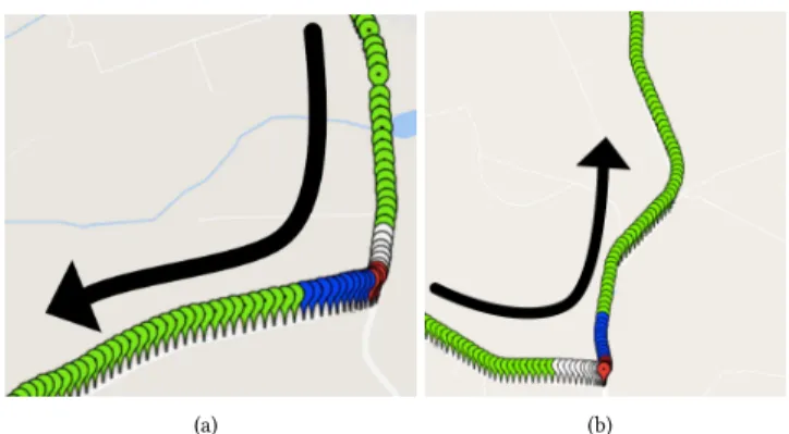
Plotting the Resulting Clusters.To validate our hypotheses, we can plot the latitude/longitude locations of the drive, along with the resulting cluster assignments. Analyzing this data, we empiri-cally discover that each of the ive clusters has a clear real-world interpretation that aligns very closely with our estimates based on the betweenness scores in Table 3. Furthermore, we notice that many consistent and repeated patterns emerge in this one hour session. For example, whenever the driver is approaching a turn, he or she follows the same sequence of clusters: going straight, slowing down, turning, speeding up, then going straight again. We plot two typical turns in the dataset, coloring the timestamps ac-cording to their cluster assignments, in Figure 5. It is important to note here that the same pattern emerges here for both left and right turns. Whereas distance-based approaches would treat these two scenarios very diferently (since several of the sensors have completely opposite values), TICC instead clusters the time series based on structural similarities. As a result, TICC assigns both left and right turns into the same underlying cluster.

8

CONCLUSION AND FUTURE WORK

(a) (b)

Figure 5: Two real-world turns in the driving session. The pin color represents cluster assignment from our TICC algo-rithm (Green = Going Straight, White = Slowing Down, Red = Turning, Blue = Speeding up). Since we cluster based on structure, rather than distance, both a left and a right turn look very similar under the TICC clustering scheme.

structure and deine each cluster by a multilayer MRF, making our results highly interpretable. To discover these clusters, TICC alternates between assigning points to clusters in a temporally consistent way, which it accomplishes through dynamic program-ming, and updating the cluster MRFs, which it does via ADMM. TICC’s promising results on both synthetic and real-world data lead to many potential directions for future research. For example, our method could be extended to learn dependency networks pa-rameterized byanyheterogeneous exponential family MRF. This would allow for a much broader class of datasets (such as boolean or categorical readings) to be incorporated into the existing TICC framework, opening up this work to new potential applications.

Acknowledgements.This work was supported by NSF IIS-1149837, NIH BD2K, DARPA SIMPLEX, DARPA XDATA, Chan Zuckerberg Biohub, SDSI, Boeing, Bosch, and Volkswagen.

REFERENCES

[1] O. Banerjee, L. El Ghaoui, and A. d’Aspremont. Model selection through sparse maximum likelihood estimation for multivariate Gaussian or binary data.JMLR, 2008.

[2] J. D. Banield and A. E. Raftery. Model-based Gaussian and non-Gaussian clus-tering.Biometrics, 1993.

[3] N. Begum, L. Ulanova, J. Wang, and E. Keogh. Accelerating dynamic time warping clustering with a novel admissible pruning strategy. InKDD, 2015.

[4] D. J. Berndt and J. Cliford. Using dynamic time warping to ind patterns in time series. InAAAI Workshop on Knowledge Disovery in Databases, 1994. [5] S. Boyd, N. Parikh, E. Chu, B. Peleato, and J. Eckstein. Distributed

optimiza-tion and statistical learning via the alternating direcoptimiza-tion method of multipliers. Foundations and Trends in Machine Learning, 2011.

[6] S. Boyd and L. Vandenberghe.Convex Optimization. Cambridge University Press, 2004.

[7] U. Brandes. A faster algorithm for betweenness centrality.Journal of Mathemati-cal Sociology, 2001.

[8] T. M. Cover and J. A. Thomas.Elements of Information Theory. John Wiley & Sons, 2012.

[9] M. Cuturi. Fast global alignment kernels. InICML, 2011.

[10] P. Danaher, P. Wang, and D. M. Witten. The joint graphical lasso for inverse covariance estimation across multiple classes.JRSS: Series B, 2014.

[11] G. Das, K.-I. Lin, H. Mannila, G. Renganathan, and P. Smyth. Rule discovery from time series. InKDD, 1998.

[12] E. Dimtriadou. Cclust: Convex clustering methods and clustering indexes. https: //CRAN.R-project.org/package=cclust, 2009.

[13] C. Fraley and A. E. Raftery. MCLUST version 3: an R package for normal mixture modeling and model-based clustering. Technical report, DTIC Document, 2006.

[14] J. Friedman, T. Hastie, and R. Tibshirani. Sparse inverse covariance estimation with the graphical lasso.Biostatistics, 2008.

[15] A. Gionis and H. Mannila. Finding recurrent sources in sequences. InRECOMB, 2003.

[16] R. M. Gray. Toeplitz and circulant matrices: A review.Foundations and Trends in Communications and Information Theory, 2006.

[17] D. Hallac, P. Nystrup, and S. Boyd. Greedy Gaussian segmentation of multivariate time series.arXiv preprint arXiv:1610.07435, 2016.

[18] T. Hastie, R. Tibshirani, and J. Friedman.The Elements of Statistical Learning. Springer, 2009.

[19] M. R. Hestenes. Multiplier and gradient methods.Journal of Optimization Theory and Applications, 1969.

[20] J. Himberg, K. Korpiaho, H. Mannila, J. Tikänmaki, and H. T. Toivonen. Time series segmentation for context recognition in mobile devices. InICDM, 2001. [21] C.-J. Hsieh, M. A. Sustik, I. S. Dhillon, and P. Ravikumar. QUIC: quadratic

approximation for sparse inverse covariance estimation.JMLR, 2014. [22] C.-J. Hsieh, M. A. Sustik, I. S. Dhillon, P. K. Ravikumar, and R. Poldrack. BIG &

QUIC: Sparse inverse covariance estimation for a million variables. InNIPS, 2013. [23] E. Keogh. Exact indexing of dynamic time warping. InVLDB, 2002.

[24] E. Keogh, J. Lin, and W. Truppel. Clustering of time series subsequences is meaningless: Implications for previous and future research. InICDM, 2003. [25] E. Keogh and M. J. Pazzani. Scaling up dynamic time warping for datamining

applications. InKDD, 2000.

[26] D. Koller and N. Friedman.Probabilistic Graphical Models: Principles and Tech-niques. MIT press, 2009.

[27] S. L. Lauritzen.Graphical models. Clarendon Press, 1996.

[28] Y. Li, J. Lin, and T. Oates. Visualizing variable-length time series motifs. InSIAM, 2012.

[29] J. Lin, E. Keogh, S. Lonardi, and B. Chiu. A symbolic representation of time series, with implications for streaming algorithms. InSIGMOD workshop on Research issues in data mining and knowledge discovery, 2003.

[30] J. Lin, E. Keogh, L. Wei, and S. Lonardi. Experiencing SAX: a novel symbolic representation of time series.Data Mining and knowledge discovery, 2007. [31] T. M. Martinetz, S. G. Berkovich, and K. J. Schulten. ’Neural-gas’ network for

vector quantization and its application to time-series prediction.IEEE Transactions on Neural Networks, 1993.

[32] C. Miyajima, Y. Nishiwaki, K. Ozawa, T. Wakita, K. Itou, K. Takeda, and F. Itakura. Driver modeling based on driving behavior and its evaluation in driver identii-cation.Proceedings of the IEEE, 2007.

[33] K. Mohan, P. London, M. Fazel, D. Witten, and S.-I. Lee. Node-based learning of multiple Gaussian graphical models.JMLR, 2014.

[34] F. Mörchen, A. Ultsch, and O. Hoos. Extracting interpretable muscle activation patterns with time series knowledge mining.International Journal of Knowledge-based and Intelligent Engineering Systems, 2005.

[35] A. Namaki, A. Shirazi, R. Raei, and G. Jafari. Network analysis of a inancial market based on genuine correlation and threshold method. Physica A: Stat. Mech. Apps., 2011.

[36] B. O’Donoghue, E. Chu, N. Parikh, and S. Boyd. Conic optimization via operator splitting and homogeneous self-dual embedding.Journal of Optimization Theory and Applications, 2016.

[37] N. Parikh and S. Boyd. Proximal algorithms.Foundations and Trends in Optimiza-tion, 2014.

[38] J. Pärkkä, M. Ermes, P. Korpipää, J. Mäntyjärvi, J. Peltola, and I. Korhonen. Activity classiication using realistic data from wearable sensors.IEEE Transactions on information technology in biomedicine, 2006.

[39] T. Rakthanmanon, B. Campana, A. Mueen, G. Batista, B. Westover, Q. Zhu, J. Za-karia, and E. Keogh. Searching and mining trillions of time series subsequences under dynamic time warping. InKDD, 2012.

[40] P. J. Rousseeuw. Silhouettes: a graphical aid to the interpretation and validation of cluster analysis.Journal of computational and applied mathematics, 1987. [41] H. Rue and L. Held.Gaussian Markov Random Fields: Theory and Applications.

CRC Press, 2005.

[42] A. Sarda-Espinosa. Dtwclust. https://cran.r-project.org/web/packages/dtwclust/ index.html, 2016.

[43] P. Smyth. Clustering sequences with hidden Markov models.NIPS, 1997. [44] A. Viterbi. Error bounds for convolutional codes and an asymptotically optimum

decoding algorithm.IEEE Transactions on Information Theory, 1967. [45] M. J. Wainwright and M. I. Jordan. Log-determinant relaxation for approximate

inference in discrete Markov random ields.IEEE Tr. on Signal Processing, 2006. [46] M. Wytock and J. Z. Kolter. Sparse Gaussian conditional random ields:

Algo-rithms, theory, and application to energy forecasting.ICML, 2013.

[47] Y. Xiong and D.-Y. Yeung. Time series clustering with ARMA mixtures.Pattern Recognition, 2004.

[48] M. Yuan and Y. Lin. Model selection and estimation in regression with grouped variables.Journal of the Royal Statistical Society: Series B, 68:49ś67, 2006. [49] S. Zolhavarieh, S. Aghabozorgi, and Y. W. Teh. A review of subsequence time