Conditional Random Fields: An Introduction ∗
Hanna M. Wallach
February 24, 2004
1 Labeling Sequential Data
The task of assigning label sequences to a set of observation sequences arises in many fields, including bioinformatics, computational linguistics and speech recognition [6, 9, 12]. For example, consider the natural language processing task of labeling the words in a sentence with their corresponding part-of-speech (POS) tags. In this task, each word is labeled with a tag indicating its appro- priate part of speech, resulting in annotated text, such as:
(1) [PRP He] [VBZ reckons] [DT the] [JJ current] [NN account] [NN deficit] [MD will] [VB narrow] [TO to] [RB only] [# #] [CD 1.8] [CD billion] [IN in] [NNP September] [. .]
Labeling sentences in this way is a useful preprocessing step for higher natural language processing tasks: POS tags augment the information contained within words alone by explicitly indicating some of the structure inherent in language. One of the most common methods for performing such labeling and segmen- tation tasks is that of employing hidden Markov models [13] (HMMs) or proba- bilistic finite-state automata to identify the most likely sequence of labels for the words in any given sentence. HMMs are a form of generative model, that defines a joint probability distribution p(X, Y ) where X and Y are random variables respectively ranging over observation sequences and their corresponding label sequences. In order to define a joint distribution of this nature, generative mod- els must enumerate all possible observation sequences – a task which, for most domains, is intractable unless observation elements are represented as isolated units, independent from the other elements in an observation sequence. More precisely, the observation element at any given instant in time may only directly
∗University of Pennsylvania CIS Technical Report MS-CIS-04-21
depend on the state, or label, at that time. This is an appropriate assumption for a few simple data sets, however most real-world observation sequences are best represented in terms of multiple interacting features and long-range depen- dencies between observation elements.
This representation issue is one of the most fundamental problems when labeling sequential data. Clearly, a model that supports tractable inference is necessary, however a model that represents the data without making unwar- ranted independence assumptions is also desirable. One way of satisfying both these criteria is to use a model that defines a conditional probability p(Y |x) over label sequences given a particular observation sequence x, rather than a joint distribution over both label and observation sequences. Conditional models are used to label a novel observation sequence x⋆by selecting the label sequence y⋆ that maximizes the conditional probability p(y⋆|x⋆). The conditional nature of such models means that no effort is wasted on modeling the observations, and one is free from having to make unwarranted independence assumptions about these sequences; arbitrary attributes of the observation data may be captured by the model, without the modeler having to worry about how these attributes are related.
Conditional random fields [8] (CRFs) are a probabilistic framework for label- ing and segmenting sequential data, based on the conditional approach described in the previous paragraph. A CRF is a form of undirected graphical model that defines a single log-linear distribution over label sequences given a particular observation sequence. The primary advantage of CRFs over hidden Markov models is their conditional nature, resulting in the relaxation of the indepen- dence assumptions required by HMMs in order to ensure tractable inference. Additionally, CRFs avoid the label bias problem [8], a weakness exhibited by maximum entropy Markov models [9] (MEMMs) and other conditional Markov models based on directed graphical models. CRFs outperform both MEMMs and HMMs on a number of real-world sequence labeling tasks [8, 11, 15].
2 Undirected Graphical Models
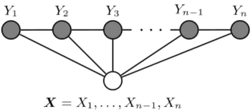
A conditional random field may be viewed as an undirected graphical model, or Markov random field [3], globally conditioned on X, the random variable representing observation sequences. Formally, we define G = (V, E) to be an undirected graph such that there is a node v ∈ V corresponding to each of the random variables representing an element Yv of Y . If each random variable Yv obeys the Markov property with respect to G, then (Y , X) is a conditional random field. In theory the structure of graph G may be arbitrary, provided it represents the conditional independencies in the label sequences being mod- eled. However, when modeling sequences, the simplest and most common graph structure encountered is that in which the nodes corresponding to elements of
Y form a simple first-order chain, as illustrated in Figure 1.
Y1 Y2 Y3
. . .
Yn−1 Yn
X = X1, . . . , Xn−1, Xn
Figure 1: Graphical structure of a chain-structured CRFs for sequences. The variables corresponding to unshaded nodes are not generated by the model.
2.1 Potential Functions
The graphical structure of a conditional random field may be used to factorize the joint distribution over elements Yvof Y into a normalized product of strictly positive, real-valued potential functions, derived from the notion of conditional independence.1 Each potential function operates on a subset of the random variables represented by vertices in G. According to the definition of conditional independence for undirected graphical models, the absence of an edge between two vertices in G implies that the random variables represented by these vertices are conditionally independent given all other random variables in the model. The potential functions must therefore ensure that it is possible to factorize the joint probability such that conditionally independent random variables do not appear in the same potential function. The easiest way to fulfill this requirement is to require each potential function to operate on a set of random variables whose corresponding vertices form a maximal clique within G. This ensures that no potential function refers to any pair of random variables whose vertices are not directly connected and, if two vertices appear together in a clique this relationship is made explicit. In the case of a chain-structured CRF, such as that depicted in Figure 1, each potential function will operate on pairs of adjacent label variables Yi and Yi+1.
It is worth noting that an isolated potential function does not have a direct probabilistic interpretation, but instead represents constraints on the configu- rations of the random variables on which the function is defined. This in turn affects the probability of global configurations – a global configuration with a high probability is likely to have satisfied more of these constraints than a global configuration with a low probability.
1The product of a set of strictly positive, real-valued functions is not guaranteed to satisfy the axioms of probability. A normalization factor is therefore introduced to ensure that the product of potential functions is a valid probability distribution over the random variables represented by vertices in G.
3 Conditional Random Fields
Lafferty et al. [8] define the the probability of a particular label sequence y given observation sequence x to be a normalized product of potential functions, each of the form
exp (X
j
λjtj(yi−1, yi, x, i) +X
k
µksk(yi, x, i)), (2)
where tj(yi−1, yi, x, i) is a transition feature function of the entire observation sequence and the labels at positions i and i − 1 in the label sequence; sk(yi, x, i) is a state feature function of the label at position i and the observation sequence; and λj and µk are parameters to be estimated from training data.
When defining feature functions, we construct a set of real-valued features b(x, i) of the observation to expresses some characteristic of the empirical dis- tribution of the training data that should also hold of the model distribution. An example of such a feature is
b(x, i) =
(1 if the observation at position i is the word “September” 0 otherwise.
Each feature function takes on the value of one of these real-valued observation features b(x, i) if the current state (in the case of a state function) or previous and current states (in the case of a transition function) take on particular val- ues. All feature functions are therefore real-valued. For example, consider the following transition function:
tj(yi−1, yi, x, i) =
(b(x, i) if yi−1= IN and yi= NNP 0 otherwise.
In the remainder of this report, notation is simplified by writing s(yi, x, i) = s(yi−1, yi, x, i)
and
Fj(y, x) =
n
X
i=1
fj(yi−1, yi, x, i),
where each fj(yi−1, yi, x, i) is either a state function s(yi−1, yi, x, i) or a transi- tion function t(yi−1, yi, x, i). This allows the probability of a label sequence y given an observation sequence x to be written as
p(y|x, λ) = 1 Z(x)exp (
X
j
λjFj(y, x)). (3)
Z(x) is a normalization factor.
4 Maximum Entropy
The form of a CRF, as given in (3), is heavily motivated by the principle of maximum entropy – a framework for estimating probability distributions from a set of training data. Entropy of a probability distribution [16] is a measure of uncertainty and is maximized when the distribution in question is as uniform as possible. The principle of maximum entropy asserts that the only probability distribution that can justifiably be constructed from incomplete information, such as finite training data, is that which has maximum entropy subject to a set of constraints representing the information available. Any other distribution will involve unwarranted assumptions. [7]
If the information encapsulated within training data is represented using a set of feature functions such as those described in the previous section, the maximum entropy model distribution is that which is as uniform as possible while ensuring that the expectation of each feature function with respect to the empirical distribution of the training data equals the expected value of that feature function with respect to the model distribution. Identifying this distribution is a constrained optimization problem that can be shown [2, 10, 14] to be satisfied by (3).
5 Maximum Likelihood Parameter Inference
Assuming the training data {(x(k), y(k))} are independently and identically dis- tributed, the product of (3) over all training sequences, as a function of the parameters λ, is known as the likelihood, denoted by p({y(k)}|{x(k)}, λ). Max- imum likelihood training chooses parameter values such that the logarithm of the likelihood, known as the log-likelihood, is maximized. For a CRF, the log- likelihood is given by
L(λ) =X
k
log 1 Z(x(k))+
X
j
λjFj(y(k), x(k))
.
This function is concave, guaranteeing convergence to the global maximum. Differentiating the log-likelihood with respect to parameter λj gives
∂L(λ)
∂λj
= Ep(Y ,X)˜ [Fj(Y , X)] − X
k
Ep(Y |x(k),λ)hFj(Y , x(k))i,
where ˜p(Y , X) is the empirical distribution of training data and Ep[·] denotes expectation with respect to distribution p. Note that setting this derivative to
zero yields the maximum entropy model constraint: The expectation of each feature with respect to the model distribution is equal to the expected value under the empirical distribution of the training data.
It is not possible to analytically determine the parameter values that maxi- mize the log-likelihood – setting the gradient to zero and solving for λ does not always yield a closed form solution. Instead, maximum likelihood parameters must be identified using an iterative technique such as iterative scaling [5, 1, 10] or gradient-based methods [15, 17].
6 CRF Probability as Matrix Computations
For a chain-structured CRF in which each label sequence is augmented by start and end states, y0 and yn+1, with labels start and end respectively, the prob- ability p(y|x, λ) of label sequence y given an observation sequence x may be efficiently computed using matrices.
Letting Y be the alphabet from which labels are drawn and y and y′ be labels drawn from this alphabet, we define a set of n + 1 matrices {Mi(x)|i = 1, . . . , n + 1}, where each Mi(x) is a |Y × Y| matrix with elements of the form
Mi(y′, y|x) = exp (X
j
λjfj(y′, y, x, i)).
The unnormalized probability of label sequence y given observation sequence x may be written as the product of the appropriate elements of the n + 1 matrices for that pair of sequences:
p(y|x, λ) = 1 Z(x)
n+1
Y
i=1
Mi(yi−1, yi|x).
Similarly, the normalization factor Z(x) for observation sequence x, may be computed from the set of Mi(x) matrices using closed semirings, an algebraic structure that provides a general framework for solving path problems in graphs. Omitting details, Z(x) is given by the (start,end) entry of the product of all n+ 1 Mi(x) matrices:
Z(x) =
"n+1 Y
i=1
Mi(x)
#
start,end
(4)
7 Dynamic Programming
In order to identify the maximum-likelihood parameter values – irrespective of whether iterative scaling or gradient-based methods are used – it must be possible to efficiently compute the expectation of each feature function with respect to the CRF model distribution for every observation sequence x(k) in the training data, given by
Ep(Y |x(k),λ)hFj(Y , x(k))i=X
y
p(Y = y|x(k), λ)Fj(y, x(k)). (5)
Performing such calculations in a na¨ıve fashion is intractable due to the required sum over label sequences: If observation sequence x(k) has n elements, there are n|Y| possible corresponding label sequences. Summing over this number of terms is prohibitively expensive.
Fortunately, the right-hand side of (5) may be rewritten as
n
X
i=1
X
y′,y
p(Yi−1 = y′, Yi= y|x(k), λ)fj(y′, y, x(k)), (6)
eliminating the need to sum over n|Y| sequences. Furthermore, a dynamic programming method, similar to the forward-backward algorithm for hidden Markov models, may be used to calculate p(Yi−1= y′, Yi = y|x(k), λ).
Defining forward and backward vectors – αi(x) and βi(x) respectively – by the base cases
α0(y|x) =
(1 if y = start 0 otherwise and
βn+1(y|x) =
(1 if y = stop 0 otherwise and the recurrence relations
αi(x)T = αi−1(x)TMi(x) and
βi(x) = Mi+1(x)βi+1(x),
the probability of Yi and Yi−1 taking on labels y′ and y given observation se- quence x(k) may be written as
p(Yi−1= y′, Yi = y|x(k), λ) = αi−1(y
′|x)M
i(y′, y|x)βi(y|x)
Z(x) .
Z(x) is given by the (start,stop) entry of the product of all n + 1 Mi(x) ma- trices as in (4). Substituting this expression into (6) yields an efficient dynamic programming method for computing feature expectations.
References
[1] A. L. Berger. The improved iterative scaling algorithm: A gentle introduc- tion, 1997.
[2] A. L. Berger, S. A. Della Pietra, and V. J. Della Pietra. A maximum en- tropy approach to natural language processing. Computational Linguistics, 22(1):39–71, 1996.
[3] P. Clifford. Markov random fields in statistics. In Geoffrey Grimmett and Dominic Welsh, editors, Disorder in Physical Systems: A Volume in Honour of John M. Hammersley, pages 19–32. Oxford University Press, 1990.
[4] T. H. Cormen, C. E. Leiserson, and R. L. Rivest. Introduction to Algo- rithms. MIT Press/McGraw-Hill, 1990.
[5] J. Darroch and D. Ratcliff. Generalized iterative scaling for log-linear mod- els. The Annals of Mathematical Statistics, 43:1470–1480, 1972.
[6] R. Durbin, S. Eddy, A. Krogh, and G. Mitchison. Biological Sequence Analysis: Probabilistic Models of Proteins and Nucleic Acids. Cambridge University Press, 1998.
[7] E. T. Jaynes. Information theory and statistical mechanics. The Physical Review, 106(4):620–630, May 1957.
[8] J. Lafferty, A. McCallum, and F. Pereira. Conditional random fields: prob- abilistic models for segmenting and labeling sequence data. In International Conference on Machine Learning, 2001.
[9] A. McCallum, D. Freitag, and F. Pereira. Maximum entropy Markov mod- els for information extraction and segmentation. In International Confer- ence on Machine Learning, 2000.
[10] S. Della Pietra, V. Della Pietra, and J. Lafferty. Inducing features of ran- dom fields. Technical Report CMU-CS-95-144, Carnegie Mellon University, 1995.
[11] D. Pinto, A. McCallum, X. Wei, and W. B. Croft. Table extraction using conditional random fields. Proceedings of the ACM SIGIR, 2003.
[12] L. Rabiner and B. H. Juang. Fundamentals of Speech Recognition. Prentice Hall Signal Processing Series. Prentice-Hall, Inc., 1993.
[13] L. R. Rabiner. A tutorial on hidden Markov models and selected applica- tions in speech recognition. Proceedings of the IEEE, 77(2):257–285, 1989. [14] A. Ratnaparkhi. A simple introduction to maximum entropy models for natural language processing. Technical Report 97-08, Institute for Research in Cognitive Science, University of Pennsylvania, 1997.
[15] F. Sha and F. Pereira. Shallow parsing with conditional random fields. Proceedings of Human Language Technology, NAACL 2003, 2003.
[16] C. E. Shannon. A mathematical theory of communication. Bell System Tech. Journal, 27:379–423 and 623–656, 1948.
[17] H. M. Wallach. Efficient training of conditional random fields. Master’s thesis, University of Edinburgh, 2002.