Munich Personal RePEc Archive
Using REIT Data to Assess the
Economic Worth of Mega-Events: The
Case of the 2020 Tokyo Olympics
Ryoh Ogawa
Osaka City University
1 May 2017
Online at https://mpra.ub.uni-muenchen.de/81025/
MPRA Paper No. 81025, posted 28 August 2017 10:45 UTC
1
Using REIT Data to Assess the Economic Worth of Mega-Events:
The Case of the 2020 Tokyo Olympics
Ryoh Ogawa Osaka City University
Abstract
This paper proposes an alternative approach by which to evaluate the effects of hosting mega-events (e.g., the Olympics, the Football World Cup, or the World Expo). Based on the capitalization hypothesis, studies within the literature have examined whether the announcement of mega-events affects the prices of firms’ stock or real estate properties. While the use of firm-level stock prices allows us to see the effects on corporate profits, using real estate property prices more comprehensively captures the effects on domestic areas inside and outside the host city. However, since the latter approach (unlike the former approach) does not involve the use of high-frequency data, it is difficult to distinguish clearly the effects that stem from related mega-events announcements. In contrast, I use data from real estate investment trusts (REITs), whose prices have the dual features of stock and property prices. Use of the standard event study methodology while using high-frequency data allows one to estimate abnormal returns accruing from the mega-event of interest; it also clarifies the relationship between return level and the characteristics of a REIT property. I present an empirical example—the 2020 Tokyo Olympics—and the results are as follows: 1) investors assessed that the comprehensive effects would be positive, 2) the effect becomes smaller as the distance from the host city (Tokyo-to) increases; and 3) even in areas far from Tokyo-to, real estate used for hotels and commercial facilities are relatively susceptible to the effects of hosting the Olympics.
Keywords: mega-events; Olympic games; real estate investment trust; event study, Japan
Graduate School of Economics, Osaka City University; [email protected]; 3-3-138 Sugimoto Sumiyoshi- ku, Osaka-shi, 558-8585 JAPAN
2 1. Introduction
How much value is inherent in hosting a global mega-event such as the Olympics, the Football World Cup, or the World Expo? Such prestigious projects tend to be seen as an honor by the host citizens, but they do require considerable public funds. Usually, a large amount of national tax money is allocated to the project—that is, residents in nonhost cities and regions must also bear the event cost.Thus, the economic net benefits that a nation enjoys from hosting a mega-event are a matter of public concern.
The impact of mega-events on various economic aspects has been investigated in the literature.1 Rose and Spiegel (2011) find that hosting mega-events significantly increases national exports, and Brückner and Pappa (2015) show that the Olympics in particular has a positive impact on gross domestic product (GDP), consumption, and investment.2 In addition, other studies investigate the effects on host cities’ income and employment levels (Jasmand and Maennig 2008; Hagn and Maennig 2008, 2009; Feddersen et al. 2009; Feddersen and Maennig 2012; Miyoshi and Sasaki 2016) and on tourism (Mitchell and Stewart 2015).
According to the capitalization hypothesis, future benefits and cost flows that accrue from a mega- event should be incorporated into the present value of assets, such as firm stocks and real estate properties. Many researchers have examined whether successful Olympics bids announcements significantly affect firms’ stock prices (Berman et al. 2000; Veraros et al. 2004; Samitas et al. 2008; Leeds et al. 2009; Mirman and Sharma 2010; Sullivan and Leeds 2016). These analyses of stock price fluctuations deal only with the effects on corporate profits. On the other hand, investigating changes in property prices as a result of information on mega-events can uncover more comprehensive effects on domestic areas. Kavetsos (2012) highlights the positive impacts of the 2012 London Olympics announcement (i.e., a successful bid in 2005) on property transaction prices in the host areas (boroughs) within London and the vicinity of the main stadium.3
An approach that uses property price data, however, suffers from the removal of simultaneous shocks unrelated to the effects of mega-events; an approach that uses stock price data would easily address this problem. This is because of differences in asset liquidity. A stock is frequently traded in the exchange markets, and so its price is available in high-frequency data (e.g., day, hour, or real-time unit data). This feature reduces the risk that multiple significant shocks will occur concurrent with the announcement period. In contrast, the liquidity of real estate properties is poor, because transactions do not occur frequently; thus, following the news release on a mega-event, a reasonable time period is needed to accumulate a certain number of transaction observations. Moreover, the available time series data on property prices (e.g.,
1 See Baade and Matheson (2016) and Maennig (2017) for surveys on the effects of major sports events, including the Olympics.
2 For these studies, Maennig and Richter (2012) and Langer et al. (2017) highlight the estimation bias that stems from not considering structural economic differences between hosting countries and others (or bidding countries and others).
3 Some associated retrospective studies investigate the effects of constructing and opening sports stadiums, and use a hedonic price model with property price data (e.g., Tu 2005; Ahlfeldt and Maennig 2010).
3
transaction prices or appraisal values4) are usually of a low frequency (in general, one-year units). This suggests the high risk of multiple shocks being mixed.5
The current study proposes an alternative approach by which to assess the value of hosting mega- events, and it makes use of real estate investment trust (REIT) data. REITs are financial instruments that generally raise funds through companies that invest in income-producing real estate—that is, a REIT price has the dual features of security and a property price.6 Since REIT prices are obtained in the form of high- frequency data (like stock prices), it is possible to employ an event study methodology to measure abnormal returns due to the announcement of the mega-event of interest.7 An abnormal return would imply the comprehensive effects of holding the mega-event, because a REIT price, like a property price, represents the discounted present value of future rents from the properties in which the REIT invests and which it owns.
Additionally, the determinants of the abnormal returns level can be clarified by using the characteristics of the REIT properties. REITs create real estate portfolios in terms of property attributes, for risk diversification purposes; this implies that the portfolio of each REIT has a unique set of characteristics. It is possible to investigate the relationship between estimated abnormal returns and the characteristics of a REIT portfolio (in this case, location and intended use of properties) by estimating a cross-sectional model. I examine the effectiveness of this method by taking up the case of the 2020 Tokyo Olympics. On September 8, 2013, Tokyo won its bid to host those Olympics, and it is thought that the International Olympic Committee (IOC) announcement changed investors’ prospects on future income from the properties that Japanese REITs (J-REITs) own. The results of using event study methodology show that the prices of the J-REITs responded significantly to the IOC announcement. In addition, I find that the abnormal returns level depends on the geographical configuration of the J-REIT properties. In particular, investors expected that the Olympics would mainly affect the host city (i.e., Tokyo-to), and that the extent of the impact would gradually decrease as the greater distances from the host city. However, even in domestic areas far from the host city, the property values of hotels and commercial facilities are found to be relatively sensitive to the Olympics, compared to those of other intended use.
This study is the first to investigate the impacts of major sports events on REIT returns. Some studies address events strongly associated with a REIT itself. (See Howe and Jain 2004, for regulatory change, and Tang et al. 2016, for debt announcements for each REIT.) Others identify the effects of social and economic mega-events. (See Bredin et al. 2007, for monetary policy; and Glascock and Lu-Andrews 2015, for
4 The values of non-traded properties are greatly appraised referring to the actual transaction prices of neighboring properties. Due to the expense, the frequency of such updates is usually once a year.
5 Even with difference-in-differences method, this problem owing to low liquidity (or low-frequent data) cannot be completely addressed. Because this method does not cope with anything against other shocks unrelated to the shock of interest for analysis, common to all sample units belong to the treatment group (or control group).
6 There are some studies investigating whether the fundamental value of the J-REIT is determined by the real estate price and/or the stock price. For J-REITs, see, for example, Miyakoshi et al. (2016).
7 The event study methodology supposes that the effects of an event will reflect immediately in security prices, assuming rationality in the marketplace (MacKinlay 1997).
4
extreme market-related events such as the Lehman Brothers bankruptcy.) This study contributes to the latter research stream; however, it is also the first study to examine the relationship between the extent of a shock and the characteristics (e.g., location and intended use) of REIT properties.8
The remainder of this paper is organized as follows. Section 2 shows the J-REITs’ returns before and after the Tokyo 2020 Olympics announcement, and then goes on to describe the use of the normal event study method. Section 3 investigates the relationship between the change in returns and the J-REITs’ characteristics, and Section 4 concludes.
2. Effect of announcement of the 2020 Tokyo Olympics on J-REIT returns
This section first describes some features of the market and of J-REIT investment properties. Second, it preliminarily states how J-REIT returns changed when Tokyo-to won the bid to host the 2020 Olympics and Paralympics. Finally, I calculate the abnormal returns for individual J-REIT prices on the first trading day immediately following the bid announcement, and test the null hypothesis that the extent of abnormal returns is not really “abnormal”: the average of the abnormal returns is zero.
2.1 The Features of the J-REIT market and J-REIT investment properties
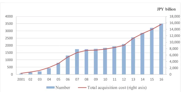
The J-REIT market developed rapidly between 2001 and 2016. J-REITs were established in September 2001, comprising two companies; their market capitalization at the end of 2001 was JPY 222 billion. At the end of 2016, however, J-REITs comprised 57 companies, and their market capitalization at the end of that year was JPY 12,123 billion.9 J-REITs comprise the largest REIT market in the world after the United States and Australia: as of November 2014, the number of REITs in the United States was 231; in Australia, 52; and in Japan, 46. Market capitalization (in USD millions) in the United States was 82,549; in Australia, 86,169; and in Japan, 84,100.10
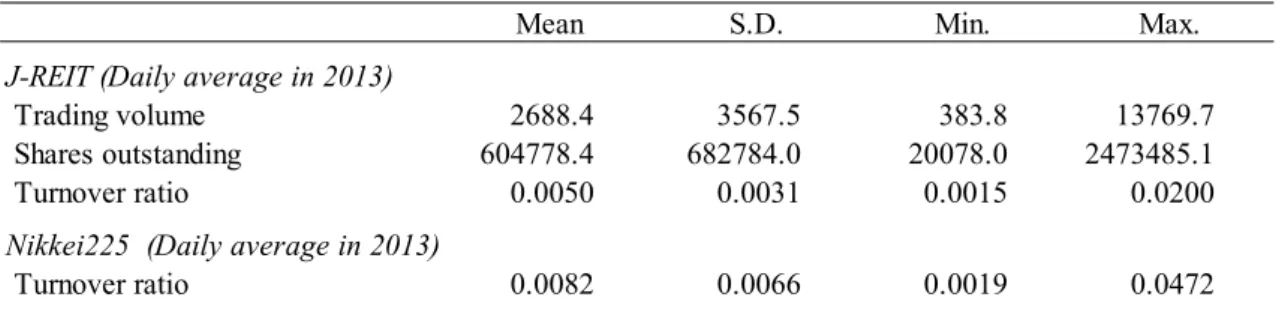
How frequently are J-REIT securities traded on the stock market? Table 1 shows the distribution of the daily average (trading-day base in 2013) of trading volume, shares outstanding, and turnover ratio for the 41 J-REITs, and the securities belonging to the Nikkei 225 (the so-called Nikkei Stock Average) that had listed at the end of August 2013.11 The turnover ratio on any given day is defined as the trading volume divided by the shares outstanding on that day; I use the turnover ratio as an indicator of security liquidity.12 The mean value of the daily average turnover ratios for the 41 J-REITs is 0.0050, and the standard deviation is 0.0031. These values are about one-half those of securities belonging to the Nikkei 225, which are listed
8 The purpose of the study of Glascock and Lu-Andrews (2015) is to clarify how REIT liquidity and size determine the extent of abnormal returns as a result of extreme market-related events.
9 This information on J-REITs is obtained from the Association for Real Estate Securitization (ARES) J-REIT Databook (http://j-reit.jp/statistics/).
10 See Table 1 in Miyakoshi et al. (2016), wherein the data source is the EPRA Global REIT Survey (2014) of the European Public Real Estate Association.
11 These 41 J-REITs are also used later, to investigate the effect of the 2020 Tokyo Olympics. Their names and security codes are summarized in Table 3.
12 Glascock and Lu-Andrews (2015) also use the turnover ratio as an indicator of REIT liquidity.
5
stocks with active trading and high liquidity selected from the listed stocks of the first section of the Tokyo Stock Exchange.
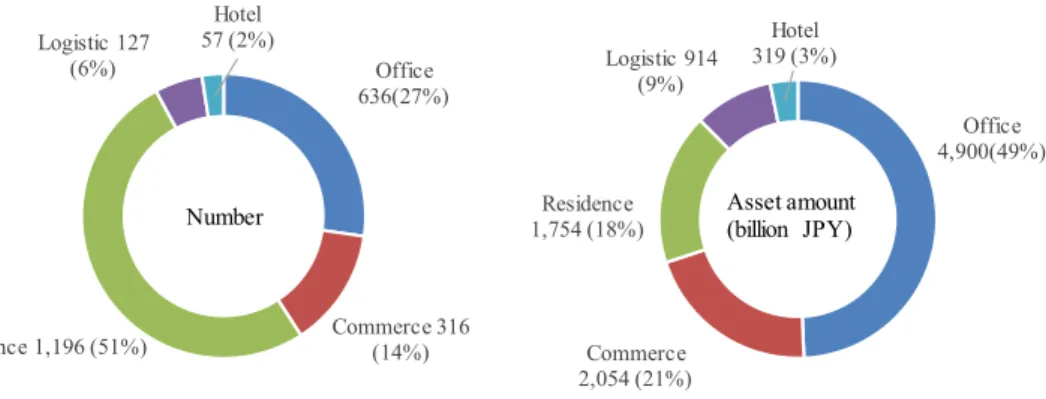
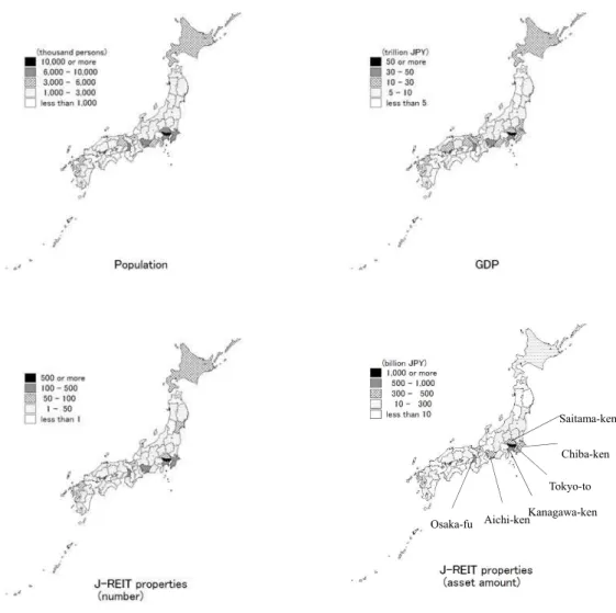
The number of real estate properties that J-REIT companies have acquired and own has also increased; Figure 1 shows the number and total acquisition cost of properties each year. In general, information on the individual properties within J-REITs is found in the settlement of accounts of each J-REIT investment company. In the case of Japan, the Association for Real Estate Securitization (ARES) constructs and discloses the J-REIT Property Database, which includes various types of attributes of the real estate properties, including location, market value, intended use (i.e., purpose of use), and age.13 Figure 2 shows the number and asset value of J-REIT properties by intended use—namely, residences, hotels, offices, commercial facilities, and logistics facilities. The proportions of properties used as residences, commercial facilities, and offices are considerably larger than those used as logistics facilities or hotels, in terms of number and asset value. The number of properties used as residences is the largest, followed by commercial facilities and offices. In contrast, the asset value of properties used as offices is the largest, followed by commercial facilities and residences. Figure 3 shows the geographical distribution of population, GDP, and J-REIT properties, by prefecture.14 J-REIT properties are found in most areas of Japan, but are heavily concentrated in certain prefectures—especially Tokyo-to, Kanagawa-ken, Chiba-ken, Saitama-ken, Osaka- fu, and Aichi-ken, whose population and GDP figures are relatively high among those in Japan.
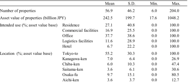
For the sake of risk diversification, REITs are likely to construct real estate portfolios while bearing in the mind property attributes; the portfolio of each REIT will therefore bear a unique set of characteristics. Table 2 reports the features of each J-REIT’s portfolio properties. The mean proportion of value by intended use (i.e., asset value base) are as follows: 37.7% for offices, 27.1% for residences, 16.9% for commercial facilities, 11.6% for logistics facilities, and 6.7% for hotels. Additionally, the standard deviation, minimum, and maximum values indicate that each proportion value varies widely across the J-REITs. As for proportion of value by prefecture (asset value base), the mean values in the key areas are as follows: 55.2% for Tokyo-to, 9.7% for Osaka-fu, 7.0% for Kanagawa-ken, 6.0% for Chiba-ken, 3.6% for Saitama-ken, and 3.6% for Aichi-ken. It is clear that most of the J-REIT companies tend to invest in and own real estate located in Tokyo-to. Additionally, the magnitude of the proportion of properties in Tokyo-to varies greatly across the J-REITs, as the standard deviation of Tokyo-to’s proportion is much larger than that of the other prefectures listed in Table 2.
2.2 Tokyo’s 2020 Olympics bid win and J-REIT returns
On September 8, 2013, it was announced that Tokyo-to would host the 2020 summer Olympics and Paralympics. In spite of failing to secure the 2016 summer Olympics, Tokyo-to continued to engage in
13 The ARES J-REIT Property Database is available from the ARES website (https://jreit-pdb.ares.or.jp/pdb/).
14 The prefecture is the first level of administrative division in Japan. There are 47 prefectures, and the name of each has “ken,” “fu,” “to,” or “do” appended to it.
6
invitation activities, and appealed to the idea of a geographically compact games: most of the competitions would take place within 8 km of the athletes’ village. It is thought that the IOC announcement changed investors’ prospects regarding future income from properties inside and outside Tokyo-to, and guided them towards those that the J-REITs owned. Incidentally, OddsChecker.com, a website for UK bookmakers, announced on September 3, 2013 that Tokyo-to had a 44% chance of winning the Olympics bid.15 Thus, it is likely that investors predicted that the chances of Tokyo’s victory or defeat were even. Consequently, the Olympic games site decision probably forced investors to change their investment portfolio including J- REITs.16 Here, I check the movement of J-REIT prices around the day when Tokyo-to won that bid.
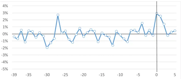
The award day was a Sunday (i.e., a nontrading day in Japan); thus, I assume that J-REIT returns responses to the announcement would occur on the first trading day thereafter. For this analysis, I set September 9, 2013 as the event day; on that day, all 41 J-REITs were trading on the Tokyo Stock Exchange. Figure 4(a) shows the daily change in the average value over the 41 J-REITs’ returns around the event day (i.e., 39 pre-event trading days, the aforementioned event trading day, and five post-event trading days).17 I find that the average value on the event day is 2.9%—an apparently large change compared to the previous day. In addition, no large negative value emerged in the five post-event days. Figure 4(b) shows the cumulative values of the daily average returns described in the Figure 4(a). I find that the cumulative values are negative in the pre-event days, but that the negative width sharply shrinks on the event day, and becomes (and remains) positive in the post-event days. These observations suggest that the announcement of Tokyo’s win likely significantly changed investors’ prospects regarding J-REIT properties.
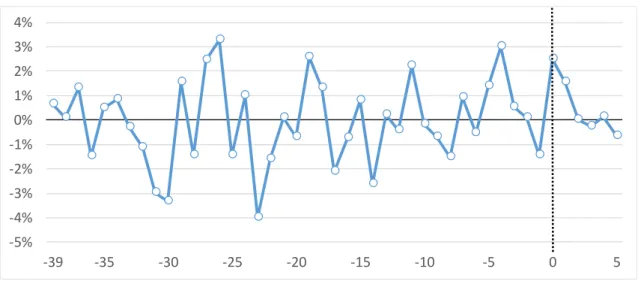
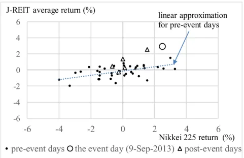
Furthermore, I also make comparisons with firm-level stock market movements. Figures 5(a) and (b) show plots of the returns for the Nikkei 225 stock index and the cumulative values, respectively. It appears that the Nikkei 225 stock index reacted to the IOC’s announcement; however, unlike with the J-REITs, the positive returns on the event day appear to be “less abnormal” than the return movements during the pre- event days. Additionally, Figure 6 is a scatterplot of the Nikkei 225 stock index’s return and the average returns of the 41 aforementioned J-REITs, for the same period. I find that the relationship on the event day (presented as a circle) seems to be an outlier compared to the stable relationships on the pre-event days. These observations imply that the impact on the J-REITs is stronger than that on the Japanese firms via the stock market.18
15 See the article in “Around The Rings” (http://aroundtherings.com/site/A__44382/Title__Istanbul-Plans-Viewing- Party-Odds-Favor-Tokyo/292/Articles).
16 On the other hand, since investors predicted that Tokyo would win with a chance of 44%, there is a possibility that prior investment was made according to the degree of the expectation for victory. Therefore, the estimation of the effects I estimate may be interpreted as the lower bound.
17 Hoshino Resort (No. 3287), one of the 41 J-REITs, was first listed on the stock market on July 12, 2013, 40 trading days prior to the event day. This is because I set July 16, 2013 (the next trading day) as the beginning of the pre-event days period.
18 Actually, Sullivan and Leeds (2016) clarify statistically that the Nikkei 225 stock index did not respond to the IOC’s announcement; they do so by estimating an autoregressive regression.
7 2.3 Calculating abnormal returns and testing hypotheses
I examine whether the announcement of the Tokyo win affected J-REIT returns—and if so, by how much— by following the standard event study methodology (e.g., MacKinlay 1997). This involves the estimation of abnormal returns and the testing of hypotheses. Abnormal returns are a measure used to evaluate the impact stemming from an event of interest, and they are calculated as the actual returns minus the normal returns in an event period. Normal returns are defined as the expected returns without being conditional on the event of interest for analysis—for example, the 2020 Olympics site decision, as seen in the case study in this study. There are two common choices for modeling normal returns: the constant mean return model and the market model. The former model assumes that the mean returns of a given security are constant through time, where the normal returns in the event period are usually calculated by averaging actual returns over the pre-event period. On the other hand, the latter model assumes a stable linear relationship between market returns and each security’s actual returns, where the normal returns in the event period are predicted thorough the linear relationship estimated in the pre-event period.
This case study focuses on results that derive from using the constant mean return model. The market model is thought to be superior to the constant mean return model with respect to removing effects due to common shocks to securities, rather than those due to the shock of interest in an event period.19 It is, however, advantageous in this case study to apply the constant mean return model, considering the possibility that mega-events can also significantly affect market returns (i.e., J-REIT market returns or firm stock market returns). If the IOC’s announcement also had a significant impact on the firm via the stock market, it would be difficult to correctly identify the extent of that impact on the J-REIT returns by using the market model. We cannot rule out the possibility, according to the preliminary observation mentioned above (see Figures 5 and 6 in subsection 2.2).
I set two length patterns for the pre-event period, to estimate the normal returns. One is July 16, 2013 to September 6, 2013 (i.e., 39 pre-event trading days); the other is June 22, 2012 to September 6, 2013 (i.e., 300 pre-event trading days); hereafter, I refer to the former period as “pattern A” and the latter period as
“pattern B.”20 Pattern A is the same as that in Figures 4 and 6 (subsection 2.2), and it is the longest span to include all the J-REITs listed on the event day (i.e., the 41 aforementioned J-REITs). On the other hand, pattern B is longer than pattern A, although the number of J-REITs therein (i.e., 35 J-REITs) is smaller. The difference in the number of J-REITs comes from the fact that six of the 41 J-REITs had not been listed for all 300 of the pre-event days.21
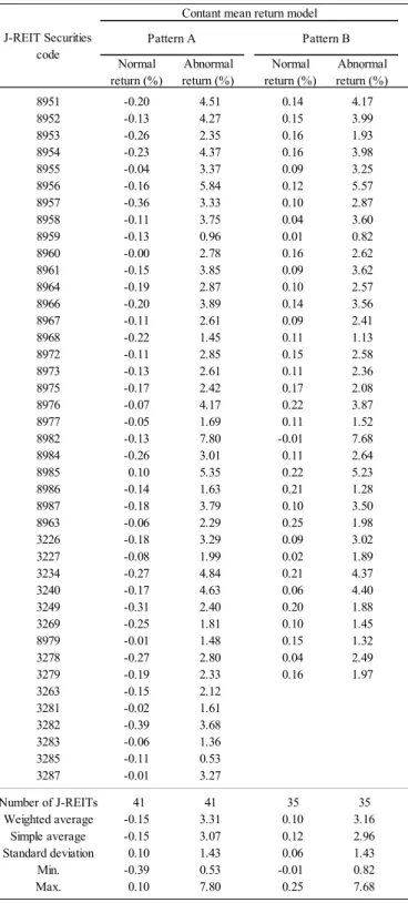
Table 4 summarizes each J-REIT’s normal and abnormal returns on the event day (September 9, 2013) according to the two aforementioned patterns (i.e., pattern A: 39 pre-event trading days, and pattern B: 300 pre-event trading days) in the constant mean return model. The weighted and simple average of abnormal
19 The noncommon (or individual) shocks to securities in an event period can be addressed by averaging abnormal returns over securities, even when we apply the constant mean return model.
20 September 6, 2013 was the trading day immediately preceding the event day.
21 MacKinlay (1997) suggests the use of more than 120 pre-event trading days.
8
returns of pattern A exceeds 3%; the maximum value is 7.80%, the minimum value is 0.53%, and the standard deviation is 1.43%. These results are almost identical to those of pattern B.
Using these estimated abnormal returns values, I conduct a t-test for the null hypothesis (i.e., that hosting the 2020 Olympics has no impact on the J-REIT returns); the simple average abnormal returns over the J-REIT securities at event day is 0. Actually, a normal t-test may lead to over-rejection when event days for each security are clustering (e.g., the extreme example is that the event day is the same for all securities, as in this study). This is because the covariances between the abnormal returns for securities will not be 0 (MacKinlay 1997). Thus, I use the adjusted test statistics proposed by Kolari and Pynnönen (2010):
, (1) where is the number of securities, and ̅ is the average of the sample cross-correlations over the pre- event days’ residuals.22 is the test statistics proposed by Boehmer et al. (1991):
√ , (2) where is the average of the event-day scaled abnormal returns ( ), and is the (cross-sectional) standard deviation of the , defined as the square root of the sample variance. is defined as the abnormal returns divided by the standard deviation of pre-event days residuals corrected by prediction error, as described by the right-hand side of equation (5) in Kolari and Pynnönen (2010).23
Table 5 presents the results of testing the hypothesis. Under the null hypothesis, the adjusted t-statistic in the constant mean return model is 2.31 for pattern A and 1.74 for pattern B, thus rejecting the null hypothesis at the 5% and 10% significance levels, respectively. These results indicate that hosting the 2020 Olympics had an impact on the J-REITs’ returns.
3. Estimating determinants of the extent of the abnormal returns
To get a sense of the magnitude of the impacts of the Tokyo 2020 Olympics on J-REITs, this section examines the relationship between the level of abnormal returns and the characteristics of J-REIT property portfolios. Specifically, I clarify whether the attributes of intended use and location influence the level of abnormal returns—and if so, how.
3.1 Cross-section regression model and construction of independent variables
I look to assess 1) the relationship between the degree of impact and the distance from the host city, 2) the relationship between the degree of impact and the intended purpose of a property, and 3) which intended use is relatively susceptible to the shock of a mega-event, even when the property is far from the host city.
22 In the case of the constant mean return model, the residual at a pre-event day for a security is calculated as the actual returns at the pre-event day minus the estimated normal returns.
23 The dominator of this right-hand side corresponds to the square root of equation (8) in MacKinlay (1997).
9
To do so, I estimate the following cross-sectional regression model (3).
∙ ∑ ∙ ∑ ∙ ∙ , (3)
where is the abnormal return for J-REIT at time τ, as obtained in the previous section; is the weighted average of distances between the host city and the location of the properties that J-REIT owns—that is, how far the J-REIT asset is from the host city; is the usage-share variable that corresponds to the share of the amount, based on market value, of real estate used for intended use k for J- REIT i; and is the disturbance term.
To build , I use the straight-line distances between the offices of two prefectural governments (i.e., Tokyo-to and the prefecture in which the property is located). The weights are the shares of asset value based on market value.
For , I classify the J-REITs’ real estate properties into five categories, as previously mentioned: residences, hotels, offices, commercial facilities, and logistics facilities. For example, if a mega- event were to increase the number of tourists, the share price of a J-REIT that invests in hotels is likely to respond to the announcement of hosting the Olympics. Furthermore, if a mega-event were to significantly improve its incomes or amenities, the share price of a J-REIT that invests in residences should also respond to it. is used as a base variable, where one of the categories must be excluded from the regression equation. (Here, I select “residence.”)
Equation (3) also includes the interaction terms ( ∙ ), whose coefficients ( ) are clues important to clarifying the third aforementioned assessment.
Table 6 presents the descriptive statistics of the independent variables. is the same as in Table 2. The mean value for is 140 km, and the standard deviation is 160 km. The minimum is 0; thus, I consider ≡ 1 for the regression.
3.2 Results
Table 7 shows the results of regression (3). Models 1 and 2 have only one type of independent variable— or , respectively—while Model 3 has both types. Additionally, Model 4 adds the interaction terms ( ∙ ) to the independent variables of Model 3.
The estimated coefficients on in Models 1, 3, and 4 are significantly negative; this means that the farther from Tokyo a property location is, the less of an impact the Olympics will make on it.
The results of the estimated coefficients on in Model 2 differ from those of Model 3. Since the adjusted R-squared of Model 3 is much better than that of Model 2, we should rely on the results of Model 3.
The coefficient on hotels in Model 3 is positive and significant at the 10% significance level: a 1% increase in the share of hotels, to replace a 1% decrease in the share of residences, increases the extent of
10
the abnormal returns (0.026%). The coefficients on offices and commercial facilities are positive and negative, respectively, but both are insignificant, even at the 10% significance level. This means that in terms of effect, they do not differ from residences. The coefficient on logistics facilities is negative and significant at the 10% significance level; a 1% increase in the share of logistics facilities, to replace a 1% decrease in the share of residences, lowers the extent of the abnormal returns (–0.009%).
The adjusted R-squared of Model 4 is better than that of Model 3; this implies the importance of considering the interaction between location and intended use. The significant value of the coefficient on in Model 4 (–1.498) supposedly measures the negative effect when real estate is fully allocated to residences; however, the results of the coefficients on ∙ show that the magnitude of this negative relationship depends on the intended use. The coefficients on these interaction terms regarding hotels and commercial facilities are positive; they are significant at the 5% and 10% significance levels, respectively. These results suggest that the magnitude of the negative relationship for hotels and for commercial facilities is weaker rather than that for residences.24 These results indicate that, even in locations far from the host city, hotels and commercial facilities are more likely to be affected by the Olympics.
4. Conclusion
Using Japanese real estate investment trust (J-REIT) data, this study proposes an alternative method for evaluating the effects of hosting mega-events. The approach using property price data targets the effects on domestic areas—more comprehensively than the approach using firm-level stock price data. However, the former approach suffers from the removal of simultaneous shocks unrelated to the mega-event. As property transactions do not occur frequently, property price data are available only at a low frequency (e.g., annual data); this feature implies the high risk of multiple shocks being mixed. In contrast, using a J-REIT price allows one to capture the features of both property and stock prices. Starting from this, I examine the impact of the 2020 Tokyo Olympics and Paralympics, using standard event study methodology. The results show that investors expect Olympics to have an impact mainly on the host city (i.e., Tokyo-to), and the extent of said impact gradually decreases as the distance from the host city increases. However, even in domestic areas far from the host city, the property values of hotels and commercial facilities are more sensitive to the Olympics than those of properties with other intended uses. As a future work, we need to compare this result of even study using J-REIT data with the associated retrospective studies.
As the REIT market grows, the number of REITs will increase and the related real estate portfolios will become richer in variety. In this context, the method described herein will become increasingly helpful for researchers to clarify the comprehensive effects of holding mega-events, and for policymakers to hold
24 Additionally, the value for offices is negative and significant at the 10% significance level.
11
mega-event as an explosive for urban and regional developments.
Acknowledgments: I am grateful for constructive comments from Yukari Iwanami, Shin Kimura, Minoru Kitahara, Wolfgang Maennig, Kenkichi Nagao, Tetsuya Nakajima, Hideki Nakamura, Akihiko Noda, Ryosuke Okazawa, Shinpei Sano, and Shuji Uranishi.
References
Ahlfeldt, G. M., & Maennig, W. (2010). Impact of sports arenas on land values: evidence from Berlin. Annals of Regional Science, 44(2), 205–227.
Baade, R. A., & Matheson, V. A. (2016). Going for the gold: The economics of the Olympics. Journal of Economic Perspectives, 30(2), 201–218.
Berman, G., Brooks, R., & Davidson, S. (2000). The Sydney Olympic games announcement and Australian stock market reaction. Applied Economics Letters, 7(12), 781–784.
Boehmer, E., Musumeci, J., & A. B. Poulsen. (1991). Event study methodology under conditions of event induced variance. Journal of Financial Economics, 30(2), 253–72.
Bredin, D., O’Reilly, G., & Stevenson, S. (2007). Monetary shocks and REIT returns. Journal of Real Estate Finance and Economics, 35(3), 315–331.
Brückner, M., & Pappa, E. (2015). News shocks in the data: Olympic games and their macroeconomic effects. Journal of Money, Credit and Banking, 47(7), 1339–1367.
Feddersen, A., Grötzinger, A. L., & Maennig, W. (2009). Investment in stadia and regional economic development—Evidence from FIFA World Cup 2006. International Journal of Sport Finance, 4(4), 221–239.
Feddersen, A., & Maennig, W. (2012). Sectoral labour market effects of the 2006 FIFA World Cup. Labor Economics, 19(6), 860–869.
Glascock, J. L., & Lu-Andrews, R. (2015). The price behavior of REITs surrounding extreme market- related events. Journal of Real Estate Finance and Economics, 51(4), 441–479.
Hagn, F., & Maennig, W. (2008). Employment effects of the Football World Cup 1974 in Germany. Labour Economics, 15(5), 1062–1075.
Hagn, F., & Maennig, W. (2009). Large sport events and unemployment: The case of the 2006 soccer World Cup in Germany. Applied Economics, 41(25), 3295–3302.
Howe, J. S., & Jain, R. (2004). The REIT Modernization Act of 1999. Journal of Real Estate Finance and Economics, 28(4), 369–388.
Jasmand, S., & Maennig, W. (2008). Regional income and employment effects of the 1972 Munich summer Olympic games. Regional Studies, 42(7), 991–1002.
Kavetsos, G. (2012). The impact of the London Olympics announcement on property prices. Urban Studies,
12 49(7), 1453–1470.
Kolari, J. W., & Pynnönen, S. (2010). Event study testing with cross-sectional correlation of abnormal returns. Review of Financial Studies, 23(11), 3996–4025.
Langer, V. C. E., Maennig, W., & Richter, F. (2017). The Olympic games as a news shock: Macroeconomic implications. Journal of Sports Economics, forthcoming: DOI: 10.1177/1527002517690788.
Leeds, M., Mirikitani, J. M., & Tang, D. (2009). Rational exuberance? An event analysis of the 2008 Olympics announcement. International Journal of Sport Finance, 4(1), 5–15.
MacKinlay, A. C. (1997). Event studies in economics and finance. Journal of Economic Literature, 35(1), 13–39.
Maennig, W. (2017). Major sports events: Economic impact. Hamburg Contemporary Economic Discussions No. 58 (Working Papers from Chair for Economic Policy, University of Hamburg). Maennig, W., & Richter, F. (2012). Exports and Olympic games: Is there a signal effect? Journal of Sports
Economics, 13(6), 635–641.
Mirman, M., & Sharma, R. (2010). Stock market reaction to Olympic games announcement. Applied Economics Letters, 17(5), 463–466.
Mitchell, H., & Stewart, M. F. (2015). What should you pay to host a party? An economic analysis of hosting sports mega-events. Applied Economics, 47(15), 1550–1561.
Miyakoshi, T., Shimada, J., & Li, K. (2016). The impacts of the 2008 and 2011 crises on the Japan REIT market. Journal of the Japanese and International Economies, 41, 30–40.
Miyoshi, K., & Sasaki, M. (2016). The long-term impacts of the 1998 Nagano winter Olympic games on economic and labor market outcomes. Asian Economic Policy Review, 11(1), 43–65.
Rose, A. K., & Spiegel, M. M. (2011). The Olympic effect. Economic Journal, 121(553), 652–677. Samitas, A., Kenourgios, D., & Zounis, P. (2008). Athens’ Olympic games 2004 impact on sponsors’ stock
returns. Applied Economics Letters, 18(19), 1569–1580.
Sullivan, C., & Leeds, M. A. (2016). Will the games pay? An event analysis of the 2020 summer Olympics announcement on stock markets in Japan, Spain, and Turkey. Applied Economics Letters, 23(12), 880– 883.
Tang, C. K, Mori, M., Ong, S. E., & Ooi, J. T. L. (2016). Debt raising and refinancing by Japanese REITs: Information content in a credit crunch. Journal of Real Estate Finance and Economics, 53(2), 141– 161.
Tu, C. C. (2005). How does a new sports stadium affect housing values? The case of Fedex Field. Land Economics, 81(3), 379–395.
Veraros, N., Kasimati, E., & Dawson, P. (2004). The 2004 Olympic games announcement and its effect on the Athens and Milan stock exchanges. Applied Economics Letters, 11(12), 749–753.
13 Figures and Tables
Figure 1 Plots of number and total acquisition cost of J-REIT properties Source: ARES J-REIT Databook (http://j-reit.jp/statistics/).
0 2,000 4,000 6,000 8,000 10,000 12,000 14,000 16,000 18,000
0 500 1000 1500 2000 2500 3000 3500 4000
2001 02 03 04 05 06 07 08 09 10 11 12 13 14 15 16
Number Total acquisition cost (right axis)
JPY billion
14
Table 1 Liquidity of J-REITs and firm stocks that belonging to Nikkei 225
Notes: I use the sample of 41 J-REITs and 222 firm stocks that belonged to the Nikkei 225 (Nikkei Average Stock) as of the end of August 2013.
Source: NEEDS Financial Quest, NIKKEI Media Marketing Inc.
Mean S.D. Min. Max.
J-REIT (Daily average in 2013)
Trading volume 2688.4 3567.5 383.8 13769.7
Shares outstanding 604778.4 682784.0 20078.0 2473485.1
Turnover ratio 0.0050 0.0031 0.0015 0.0200
Nikkei225 (Daily average in 2013)
Turnover ratio 0.0082 0.0066 0.0019 0.0472
15
Figure 2 The numbers and asset values of J-REIT properties, by intended use
Notes: Using the latest financial reports of each J-REIT at the end of August 2013 (from the ARES J-REIT Property Database [https://jreit-pdb.ares.or.jp/pdb/]), I classify the J-REIT real estate properties into five categories: Residence, Hotel, Office, Commercial facilities, and Logistics facilities. If a piece of real estate has more than two intended uses, I select that which is listed first, assuming that this is likely the primary one. The asset value is based on market value— specifically, appraisal values at that time.
Office 636(27%)
Commerce 316 (14%) Residence 1,196 (51%)
Logistic 127 (6%)
Hotel 57 (2%)
Number
Office 4,900(49%)
Commerce 2,054 (21%) Residence 1,754 (18%)
Logistic 914 (9%)
Hotel 319 (3%)
Asset amount (billion JPY)
16
Figure 3 Geographical distribution of population, GDP, and J-REIT properties, by prefecture
Notes: Population data (as of 2013) are from the Ministry of Internal Affairs and Communications. GDP data (as of 2013) are from the Cabinet Office of the government of Japan (Economic and Social Research Institute). J-REIT data are from the ARES J-REIT Property Database (as of the end of August 2013).
Tokyo-to Aichi-ken
Osaka-fu
Chiba-ken
Kanagawa-ken Saitama-ken
17
Table 2 Characteristics of J-REIT portfolio properties (at the end of August 2013)
Notes: I use the sample of 41 J-REITs listed at the end of August 2013. The asset value is based on market value— specifically, appraisal values at that time. J-REIT data are from the ARES J-REIT Property Database (as of the end of August 2013).
Mean S.D. Min. Max.
Number of properties 56.9 46.2 6.0 204.0
Asset value of properties (billlion JPY) 242.5 199.7 17.6 1048.2 Intended use (%; asset value base) Residence 27.1 40.8 0.0 100.0 Commercial facilities 16.9 25.5 0.0 100.0
Office 37.7 38.6 0.0 100.0
Logistics facilities 11.6 28.9 0.0 100.0
Hotel 6.7 22.2 0.0 100.0
Location (%; asset value base) Tokyo-to 55.2 30.3 0.0 100.0
Kanagawa-ken 7.0 6.4 0.0 26.9
Chiba-ken 6.0 10.3 0.0 47.4
Saitama-ken 3.6 6.1 0.0 30.6
Osaka-fu 9.7 15.1 0.0 80.5
Aichi-ken 3.6 3.7 0.0 12.7
18
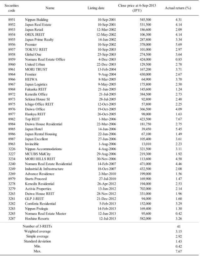
Table 3 Actual returns of 41 individual J-REITs on the event day (September 9, 2013)
Notes: The 41 J-REITs were listed on the Tokyo stock market on the event day; in this table, they are listed in order of initial listing date. The weighted averages of actual returns are calculated using the weights of the shares of close price on September 6, 2013, the trading day immediately preceding the event day.
8951 Nippon Building 10-Sep-2001 545,500 4.31
8952 Japan Real Estate 10-Sep-2001 531,500 4.14
8953 Japan Retail 12-Mar-2002 186,600 2.09
8954 ORIX JREIT 12-May-2002 106,300 4.14
8955 Japan Prime Realty 14-Jun-2002 287,800 3.34
8956 Premier 10-Sep-2002 378,000 5.69
8957 TOKYU REIT 10-Sep-2003 101,000 2.97
8958 Global One 25-Sep-2003 274,500 3.64
8959 Nomura Real Estate Office 4-Dec-2003 424,000 0.83
8960 United Urban 22-Dec-2003 129,500 2.78
8961 MORI TRUST 13-Feb-2004 167,200 3.71
8964 Frontier 9-Aug-2004 430,000 2.67
8966 HEIWA 8-Mar-2005 64,900 3.70
8967 Japan Logistics 9-May-2005 175,800 2.50
8968 Fukuoka REIT 21-Jun-2005 145,600 1.24
8972 Kenedix Office 21-Jul-2005 384,500 2.73
8973 Sekisui House SI 28-Jul-2005 92,800 2.48
8975 Ichigo Office REIT 12-Oct-2005 57,800 2.25
8976 Daiwa Office 19-Oct-2005 366,500 4.09
8977 Hankyu REIT 26-Oct-2005 98,000 1.63
8982 Top REIT 1-Mar-2006 423,500 7.67
8984 Daiwa House Residential 22-Mar-2006 181,750 2.75
8985 Japan Hotel 14-Jun-2006 39,450 5.45
8986 Japan Rental Housing 22-Jun-2006 67,100 1.49
8987 Japan Excellent 27-Jun-2006 105,400 3.61
8963 Invincible 1-Aug-2006 13,010 2.23
3226 Nippon Accommodations 4-Aug-2006 321,500 3.11
3227 MCUBS MidCity 29-Aug-2006 219,300 1.92
3234 MORI HILLS REIT 30-Nov-2006 113,600 4.58
3240 Nomura Real Estate Residential 14-Feb-2007 471,000 4.46
3249 Industrial & Infrastructure 18-Oct-2007 432,500 2.08
3269 Advance Residence 2-Mar-2010 199,000 1.56
8979 Starts Proceed 27-Jul-2010 169,900 1.47
3278 Kenedix Residential 26-Apr-2012 194,000 2.53
3279 Activia Properties 13-Jun-2012 702,000 2.14
3263 Daiwa House REIT 28-Nov-2012 331,000 1.96
3281 GLP J-REIT 21-Dec-2012 94,000 1.60
3282 Comforia Residential 5-Feb-2013 152,000 3.29
3283 Nippon Prologis 14-Feb-2013 169,400 1.30
3285 Nomura Real Estate Master 12-Jun-2013 95,600 0.42
3287 Hoshino Resorts 12-Jul-2013 582,000 3.26
41 3.15 2.921.43 0.42 7.67 Securities
code Name Listing date Close price at 6-Sep-2013
(JPY)
Number of J-REITs Simple average Weighted average Standard deviation
Actual return (%)
Max.Min.
19 (a) Average returns for J-REITs
(b) Cumulative values of the average returns for J-REITs
Figure 4 Plot of J-REIT average returns around the event day
Notes: The observation period consists of 39 pre-event days, the event day, and five post-event days; the event day (September 9, 2013) is expressed as 0. The returns of the 41 J-REITs, each of which was traded on the Tokyo Stock Exchange on the event day, are calculated on a closing-price basis. J-REIT daily prices are obtained from the database of NEEDS Financial Quest, NIKKEI Media Marketing Inc.
‐5%
‐4%
‐3%
‐2%
‐1% 0% 1% 2% 3% 4%
‐39 ‐35 ‐30 ‐25 ‐20 ‐15 ‐10 ‐5 0 5
‐9%‐8%
‐7%‐6%
‐5%‐4%
‐3%‐2%
‐1% 0% 1% 2% 3%
‐39 ‐35 ‐30 ‐25 ‐20 ‐15 ‐10 ‐5 0 5
20 (a) Average returns for Nikkei 225
(b) Cumulative values of the average returns for Nikkei 225
Figure 5 Nikkei 225 (Nikkei Stock Average) returns around the event day
Notes: The observation period is identical to that of Figure 2. The daily Nikkei 225 prices are obtained from the database of NEEDS Financial Quest, NIKKEI Media Marketing Inc.
‐5%
‐4%
‐3%
‐2%
‐1% 0% 1% 2% 3% 4%
‐39 ‐35 ‐30 ‐25 ‐20 ‐15 ‐10 ‐5 0 5
‐9%‐8%
‐7%‐6%
‐5%‐4%
‐3%‐2%
‐1% 0% 1% 2% 3%
‐39 ‐35 ‐30 ‐25 ‐20 ‐15 ‐10 ‐5 0 5
21
Figure 6 Scatterplot of Nikkei 225 returns and the J-REIT average returns around the event day.
Notes: The daily Nikkei 225 prices are obtained from the database of NEEDS Financial Quest, NIKKEI Media Marketing Inc. The figure uses the sample of the 41 J-REITs that were listed during all 39 pre-event days.
-6 -4 -2 0 2 4 6
-6 -4 -2 0 2 4 6
pre-event days the event day (9-Sep-2013) post-event days
J-REIT average return (%)Nikkei 225 return (%) linear approximation for pre-event days
22 Table 4 Normal and abnormal returns on the event day
Notes: Abnormal returns for a J-REIT on the event day are calculated as actual returns on the event day minus normal returns on the event day. The normal return on the event day is calculated following the constant mean return model of the standard event study method (e.g., MacKinlay 1997). Weighted averages are calculated using the weights of the shares of closing price on the trading day preceding the event day.
Normal
return (%) return (%)Abnormal return (%)Normal return (%)Abnormal
8951 -0.20 4.51 0.14 4.17
8952 -0.13 4.27 0.15 3.99
8953 -0.26 2.35 0.16 1.93
8954 -0.23 4.37 0.16 3.98
8955 -0.04 3.37 0.09 3.25
8956 -0.16 5.84 0.12 5.57
8957 -0.36 3.33 0.10 2.87
8958 -0.11 3.75 0.04 3.60
8959 -0.13 0.96 0.01 0.82
8960 -0.00 2.78 0.16 2.62
8961 -0.15 3.85 0.09 3.62
8964 -0.19 2.87 0.10 2.57
8966 -0.20 3.89 0.14 3.56
8967 -0.11 2.61 0.09 2.41
8968 -0.22 1.45 0.11 1.13
8972 -0.11 2.85 0.15 2.58
8973 -0.13 2.61 0.11 2.36
8975 -0.17 2.42 0.17 2.08
8976 -0.07 4.17 0.22 3.87
8977 -0.05 1.69 0.11 1.52
8982 -0.13 7.80 -0.01 7.68
8984 -0.26 3.01 0.11 2.64
8985 0.10 5.35 0.22 5.23
8986 -0.14 1.63 0.21 1.28
8987 -0.18 3.79 0.10 3.50
8963 -0.06 2.29 0.25 1.98
3226 -0.18 3.29 0.09 3.02
3227 -0.08 1.99 0.02 1.89
3234 -0.27 4.84 0.21 4.37
3240 -0.17 4.63 0.06 4.40
3249 -0.31 2.40 0.20 1.88
3269 -0.25 1.81 0.10 1.45
8979 -0.01 1.48 0.15 1.32
3278 -0.27 2.80 0.04 2.49
3279 -0.19 2.33 0.16 1.97
3263 -0.15 2.12
3281 -0.02 1.61
3282 -0.39 3.68
3283 -0.06 1.36
3285 -0.11 0.53
3287 -0.01 3.27
Number of J-REITs 41 41 35 35
Weighted average -0.15 3.31 0.10 3.16
Simple average -0.15 3.07 0.12 2.96
Standard deviation 0.10 1.43 0.06 1.43
Min. -0.39 0.53 -0.01 0.82
Max. 0.10 7.80 0.25 7.68
Pattern A Pattern B
J-REIT Securities code
Contant mean return model
23 Table 5 Results of hypothesis tests
Notes: Abnormal returns for a J-REIT on the event day are calculated as actual returns on the event day minus normal returns on the event day. The normal return on the event day is calculated following the constant mean return model of the standard event study methodology (e.g., MacKinlay 1997). I set two patterns for the pre-event period to estimate the normal returns: pattern A is July 16, 2013 to September 6, 2013, and Pattern B is June 22, 2012 to September 6, 2013. The values above the parentheses are averages over the 41 J-REITs that correspond to all the J-REITs listed on the event day, or over the 35 J-REITs that continued to list over the period of pattern B. The values in parentheses are adjusted t-statistics proposed by Kolari and Pynnönen (2010), to control for cross-correlation between abnormal returns. Significantly different from zero at *90% confidence, **95% confidence, ***99% confidence.
3.07 ** 2.96 *
(2.31) (1.74)
Average of abnormal returns
Pattern A Pattern B
24 Table 6 Descriptive statistics for independent variables
Mean S.D. Min. Max.
WAD (100km) 1.4 1.6 0 8.7
USAGEk (%) Residence 27.1 40.8 0 100.0
Hotel 6.7 22.2 0 100.0
Office 37.7 38.6 0 100.0
Commercial facilities 16.9 25.5 0 100.0
Logistics facilities 11.6 28.9 0 100.0
25 Table 7 Cross-sectional model
Notes: The estimation method for regression (3) is least squares. Robust standard errors used to correct for heteroskedasticity are in squared brackets.
Significantly different from zero at *90% confidence, **95% confidence, ***99% confidence.
-1.349 ** -1.594 *** -1.498 **
[0.578] [0.520] [0.622]
USAGEk Hotel 0.011 0.026 * -0.014
[0.009] [0.015] [0.013]
Office 0.011 * 0.007 0.021 **
[0.006] [0.005] [0.009]
Commercial -0.011 * -0.001 -0.022
[0.006] [0.008] [0.014]
Logistics -0.013 ** -0.009 * -0.018
[0.005] [0.005] [0.020]
log(WAD)*USAGEk Hotel 0.027 **
[0.011]
Office -0.026 *
[0.015]
Commercial 0.021 *
[0.013]
Logistics 0.011
[0.019]
Constant 4.059 *** 2.910 *** 3.908 *** 3.848 ***
[0.464] [0.335] [0.464] [0.432]
Adj-R-squared 0.185 0.193 0.367 0.482
Sample size 41 41 41 41
log(WAD)
model 1 model 2 model 3 model 4