Improving Lexical Choice in Neural Machine Translation
Toan Q. Nguyen and David Chiang Department of Computer Science and Engineeering
University of Notre Dame
{tnguye28,dchiang}@nd.edu
Abstract
We explore two solutions to the problem of mistranslating rare words in neural ma-chine translation. First, we argue that the standard output layer, which computes the inner product of a vector representing the context with all possible output word em-beddings, rewards frequent words dispro-portionately, and we propose to fix the norms of both vectors to a constant value. Second, we integrate a simple lexical mod-ule which is jointly trained with the rest of the model. We evaluate our approaches on eight language pairs with data sizes rang-ing from 100k to 8M words, and achieve improvements of up to +4.5 BLEU, sur-passing phrase-based translation in nearly all settings.
1 Introduction
Neural network approaches to machine translation (Sutskever et al., 2014; Bahdanau et al., 2015; Lu-ong et al., 2015a; Gehring et al., 2017) are appeal-ing for their sappeal-ingle-model, end-to-end trainappeal-ing pro-cess, and have demonstrated competitive perfor-mance compared to earlier statistical approaches (Koehn et al., 2007; Junczys-Dowmunt et al., 2016). However, there are still many open prob-lems in NMT (Koehn and Knowles, 2017). One particular issue is mistranslation of rare words. For example, consider the Uzbek sentence:
Source: Ammo muammolar hali ko’p, deydi amerikalik olim Entoni Fauchi.
Reference:But still there are many problems, says American scientist Anthony Fauci.
Baseline NMT:But there is still a lot of problems, says James Chan.
At the position where the output should beFauci, the NMT model’s top three candidates areChan,
Fauci, and Jenner. All three surnames occur in the training data with reference to immunologists: Fauci is the director of the National Institute of Allergy and Infectious Diseases, Margaret (not James) Chan is the former director of the World Health Organization, and Edward Jenner invented smallpox vaccine. But Chan is more frequent in the training data than Fauci, and James is more frequent than eitherAnthonyorMargaret.
Because NMT learns word representations in continuous space, it tends to translate words that “seem natural in the context, but do not reflect the content of the source sentence” (Arthur et al., 2016). This coincides with other observations that NMT’s translations are often fluent but lack accu-racy (Wang et al., 2017; Wu et al., 2016).
Why does this happen? At each time step, the model’s distribution over output wordseis
p(e)∝expWe·h˜ +be
whereWeandbe are a vector and a scalar
depend-ing only on e, and ˜h is a vector depending only on the source sentence and previous output words. We propose two modifications to this layer. First, we argue that the termWe·h˜, which measures how
wellefits into the context ˜h, favors common words disproportionately, and show that it helps to fix the norm of both vectors to a constant. Second, we add a new term representing a more direct connection from the source sentence, which allows the model to better memorize translations of rare words.
Below, we describe our models in more de-tail. Then we evaluate our approaches on eight language pairs, with training data sizes ranging from 100k words to 8M words, and show improve-ments of up to +4.5 BLEU, surpassing phrase-based translation in nearly all settings. Finally, we provide some analysis to better understand why our modifications work well.
ha-en tu-en hu-en
untied embeddings 17.2 11.5 26.5 tied embeddings 17.4 13.8 26.5
don’t normalize ˜ht 18.6 14.2 27.1
normalize ˜ht 20.5 16.1 28.8
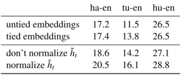
Table 1: Preliminary experiments show that ty-ing target embeddty-ings with output layer weights performs as well as or better than the baseline, and that normalizing ˜h is better than not normal-izing ˜h. All numbers are BLEU scores on devel-opment sets, scored against tokenized references.
2 Neural Machine Translation
Given a source sequence f = f1f2· · ·fm, the
goal of NMT is to find the target sequence e = e1e2· · ·enthat maximizes the objective function:
logp(e| f)=
n
X
t=1
logp(et |e<t,f).
We use the global attentional model with gen-eral scoring function and input feeding by Lu-ong et al. (2015a). We provide only a very brief overview of this model here. It has an encoder, an attention, and a decoder. The encoder converts the words of the source sentence into word em-beddings, then into a sequence of hidden states. The decoder generates the target sentence word by word with the help of the attention. At each time step t, the attention calculates a set of attention weights at(s). These attention weights are used to
form a weighted average of the encoder hidden states to form a context vector ct. From ct and
the hidden state of the decoder are computed the
attentional hidden stateh˜t. Finally, the predicted
probability distribution of thet’th target word is:
p(et |e<t,f)=softmax(Woh˜t+bo). (1)
The rows of the output layer’s weight matrixWo
can be thought of as embeddings of the output vo-cabulary, and sometimes are in fact tied to the em-beddings in the input layer, reducing model size while often achieving similar performance (Inan et al., 2017; Press and Wolf, 2017). We verified this claim on some language pairs and found out that this approach usually performs better than without tying, as seen in Table 1. For this reason, we always tie the target embeddings andWoin all of our models.
3 Normalization
The output word distribution (1) can be written as:
p(e)∝expkWek kh˜kcosθWe,h˜+be
,
whereWe is the embedding ofeandbeis thee’th
component of the biasbo; and θW
e,h˜ is the angle betweenWeand ˜h. We can intuitively interpret the
terms as follows. The term kh˜k has the effect of sharpening or flattening the distribution, reflect-ing whether the model is more or less certain in a particular context. The cosine similarity cosθW
e,˜h measures how wellefits into the context. The bias
be controls how much the word e is generated; it
is analogous to the language model in a log-linear translation model (Och and Ney, 2002).
Finally,kWekalso controls how muche is
gen-erated. Figure 1 shows that it generally correlates with frequency. But because it is multiplied by cosθW
e,h˜, it has a stronger effect on words whose embeddings have direction similar to ˜h, and less effect or even a negative effect on words in other directions. We hypothesize that the result is that the model learnskWekthat are disproportionately
large.
For example, returning to the example from Section 1, these terms are:
e kWek kh˜k cosθWe,h˜ be logit
Chan 5.25 19.5 0.144 −1.53 13.2 Fauci 4.69 19.5 0.154 −1.35 12.8 Jenner 5.23 19.5 0.120 −1.59 10.7
Observe thatθW
e,˜hand evenbeboth favor the cor-rect output word Fauci, whereas kWek favors the
more frequent, but incorrect, wordChan. The most frequently-mentioned immunologist trumps other immunologists.
To solve this issue, we propose to fix the norm of all target word embeddings to some valuer. We do this by projected gradient descent: after an up-date, project eachWe onto the hypersphere of
ra-diusr. Because this is an expensive operation, in practice, the projection can be performed periodi-cally instead of after every update.
A similar argument could be made forkh˜tk:
be-cause a largekh˜tksharpens the distribution,
caus-ing frequent words to more strongly dominate rare words, we might want to limit it as well. We com-pared both approaches on a development set and found that replacing ˜ht in equation (1) with kh˜rtkh˜t
2 4 6 8
k
We
k
ha-en tu-en hu-en
0 5,000 10,000 15,000 −2
−1 0
frequency rank ofe
be
ha-en tu-en hu-en
Figure 1: The word embedding normkWek
gener-ally correlates with the frequency ofe, except for the most frequent words. The bias be has the
op-posite behavior. The plots show the median and range of bins of size 256.
For the sake of brevity, from now on, we use the termnormalizationto mean projection onto the hypersphere of radiusr, whether by projected gra-dient descent or by modifying the model itself.
4 Lexical Translation
The attentional hidden state ˜h contains informa-tion not only about the source word(s) correspond-ing to the current target word, but also the texts of those source words and the preceding con-text of the target word. This could make the model prone to generate a target word that fits the context but doesn’t necessarily correspond to the source word(s). Count-based statistical models, by con-trast, don’t have this problem, because they sim-ply don’t model any of this context. Arthur et al. (2016) try to alleviate this issue by integrating a count-based lexicon into an NMT system. How-ever, this lexicon must be trained separately using GIZA++(Och and Ney, 2003), and its parameters form a large, sparse array, which can be difficult to store in GPU memory.
We propose instead to use a simple feedforward
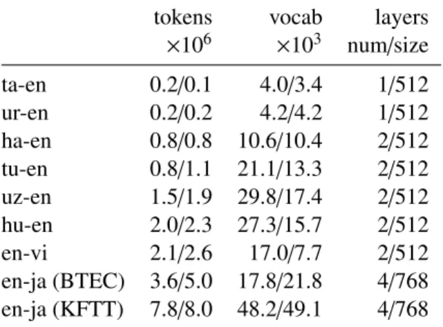
tokens vocab layers ×106 ×103 num/size ta-en 0.2/0.1 4.0/3.4 1/512 ur-en 0.2/0.2 4.2/4.2 1/512 ha-en 0.8/0.8 10.6/10.4 2/512 tu-en 0.8/1.1 21.1/13.3 2/512 uz-en 1.5/1.9 29.8/17.4 2/512 hu-en 2.0/2.3 27.3/15.7 2/512 en-vi 2.1/2.6 17.0/7.7 2/512 en-ja (BTEC) 3.6/5.0 17.8/21.8 4/768 en-ja (KFTT) 7.8/8.0 48.2/49.1 4/768
Table 2: Statistics of data and models: eff ec-tive number of training source/target tokens, source/target vocabulary sizes, number of hidden layers and number of units per layer.
neural network (FFNN) that is trained jointly with the rest of the NMT model to generate a target word based directly on the source word(s). Let fs
(s = 1, . . . ,m) be the embeddings of the source words. We use the attention weights to form a weighted average of the embeddings (not the hid-den states, as in the main model) to give an aver-age source-word embedding at each decoding time stept:
ftℓ =tanhX
s
at(s)fs.
Then we use a one-hidden-layer FFNN with skip connections (He et al., 2016):
hℓt =tanh(W ftℓ)+ ftℓ
and combine its output with the decoder output to get the predictive distribution over output words at time stept:
p(yt|y<t,x)=softmax(Woh˜t+bo+Wℓhℓt +b
ℓ ).
For the same reasons that were given in Sec-tion 3 for normalizing ˜ht and the rows ofWto, we
normalize hℓt and the rows of Wℓ as well. Note, however, that we do not tie the rows of Wℓ with the word embeddings; in preliminary experiments, we found this to yield worse results.
5 Experiments
5.1 Data
We evaluated our approaches on various language pairs and datasets:
• Tamil (ta), Urdu (ur), Hausa (ha), Turkish (tu), and Hungarian (hu) to English (en), us-ing data from the LORELEI program.
• English to Vietnamese (vi), using data from the IWSLT 2015 shared task.1
• To compare our approach with that of Arthur et al. (2016), we also ran on their English to Japanese (ja) KFTT and BTEC datasets.2
We tokenized the LORELEI datasets using the default Moses tokenizer, except for Urdu-English, where the Urdu side happened to be tokenized us-ing Morfessor FlatCat (w = 0.5). We used the preprocessed Vietnamese and English-Japanese datasets as distributed by Luong et al., and Arthur et al., respectively. Statistics about our data sets are shown in Table 2.
5.2 Systems
We compared our approaches against two baseline NMT systems:
untied, which does not tie the rows ofWo to the
target word embeddings, and tied, which does.
In addition, we compared against two other base-line systems:
Moses: The Moses phrase-based translation sys-tem (Koehn et al., 2007), trained on the same data as the NMT systems, with the same maximum sen-tence length of 50. No additional data was used for training the language model. Unlike the NMT systems, Moses used the full vocabulary from the training data; unknown words were copied to the target sentence.
Arthur:Our reimplementation of the discrete lex-icon approach of Arthur et al. (2016). We only tried theirautolexicon, using GIZA++(Och and Ney, 2003), integrated using theirbiasapproach.
Against these baselines, we compared our new systems:
fixnorm: The normalization approach described in Section 3.
1https://nlp.stanford.edu/projects/nmt/ 2http://isw3.naist.jp/~philip-a/emnlp2016/
fixnorm+lex: The same, with the addition of the lexical translation module from Section 4.3
5.3 Details
Model For all NMT systems, we fed the source sentences to the encoder in reverse order during both training and testing, following Luong et al. (2015a). Information about the number and size of hidden layers is shown in Table 2. The word embedding size is always equal to the hidden layer size.
Following common practice, we trained on sen-tences of 50 tokens or less only. We limited the vocabulary to word types that appear no less than 5 times in the training data and map the rest toUNK. For the English-Japanese and English-Vietnamese datasets, we used the vocabulary sizes reported in their respective papers (Arthur et al., 2016; Luong and Manning, 2015).
Forfixnorm, we triedr ∈ {3,5,7}and selected the best value based on the development set, which was r = 5 except for English-Japanese (BTEC), where r = 7. For fixnorm+lex, because Wsh˜t +
Wℓhℓt takes on values in [−2r2,2r2], we reduced our candidatervalues by roughly a factor of √2, tor∈ {2,3.5,5}. A radiusr =3.5 seemed to work the best for all language pairs.
Training We trained all NMT systems with Adadelta (Zeiler, 2012). All parameters were ini-tialized uniformly from [−0.01,0.01]. When a gra-dient’s norm exceeded 5, we normalized it to 5. We also used dropout on non-recurrent connections only (Zaremba et al., 2014), with probability 0.2. We used minibatches of size 32. We trained for 50 epochs, validating on the development set after ev-ery epoch, except on English-Japanese, where we validated twice per epoch. We kept the best check-point according to its BLEU on the development set.
For the fixnorm (and fixnorm+lex) systems, as mentioned above, normalizing the output em-beddings is a computationally expensive operation that dramatically slows down training. For effi -ciency, we only normalized embeddings after ev-ery 10 updates.
Inference We used beam search with a beam size of 12 for translating both the development and test sets. Since NMT often favors short trans-lations (Cho et al., 2014), we followed Wu et al.
3Code for this paper can be found at
(2016) in using a modified score s(e | f) in place of log-probability:
s(e| f)= logp(e| f) lp(e)
lp(e)= (5+|e|)
α
(5+1)α
We setα=0.8 for all of our experiments.
Finally, we applied a postprocessing step to re-place each UNK in the target translation with the source word with the highest attention score (Lu-ong et al., 2015b).
Evaluation For translation into English, we re-port case-sensitive BLEU against detokenized ref-erences, computed usingmulti-bleu.perl. For English-Japanese and English-Vietnamese, we re-port tokenized, case-sensitive BLEU following Arthur et al. (2016) and Luong and Manning (2015). We measure statistical significance using bootstrap resampling (Koehn, 2004).
6 Results and Analysis 6.1 Overall
Our results are shown in Table 3. First, we ob-serve, as has often been noted in the literature, that NMT tends to perform poorer than PBMT on low resource settings (note that the rows of this table are sorted by training data size).
Our fixnorm system alone shows large improvements (shown in parentheses) rela-tive to tied. Integrating the lexical module (fixnorm+lex) adds in further gains. Our fixnorm+lex models surpass Moses on all tasks except Urdu-English, where it is 1.1 BLEU short, and English-Vietnamese, where it is only 0.06 BLEU ahead.
The method of Arthur et al. (2016) does im-prove over the baseline NMT on most language pairs, but not by as much and as consistently as our models, and often not as well as Moses. Un-fortunately, we could not replicate their approach for English-Japanese (KFTT) because the lexical table was too large to fit into the computational graph.
For English-Japanese (BTEC), we note that, due to the small size of the test set, all systems except for Moses are in fact not significantly dif-ferent from tied (p > 0.01). On all other tasks, however, our systems significantly improve over tied(p<0.01).
6.2 Impact on translation
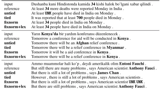
In Table 4, we show examples of typical trans-lation mistakes made by the baseline NMT sys-tems. In the Uzbek example (top), untied and tied have confused 34 with UNK and 700, while
in the Turkish one (middle), they incorrectly out-put other proper names,AfghanandMyanmar, for the proper name Kenya. Both our fixnorm and fixnorm+lex, on the other hand, translate these words correctly.
The bottom example is the one introduced in Section 1. We can see that ourfixnormapproach does not completely solve the mistranslation is-sue, since it translatesEntoni Fauchi toUNK UNK
(which is arguably better than James Chan). On the other hand, fixnorm+lex gets this right. To better understand how the lexical module helps in this case, we look at the top five translations for the wordFauciinfixnorm+lex:
e cosθW
e,h˜ cosθWel,hl be+b
l e logit
Fauci 0.522 0.762 −8.71 7.0 UNK 0.566 −0.009 −1.25 5.6 Anthony 0.263 0.644 −8.70 2.4 Ahmedova 0.555 0.173 −8.66 0.3 Chan 0.546 0.150 −8.73 −0.2 As we can see, while cosθW
e,h˜ might still be con-fused between similar words, cosθWl
e,hl signifi-cantly favorsFauci.
6.3 Alignment and unknown words
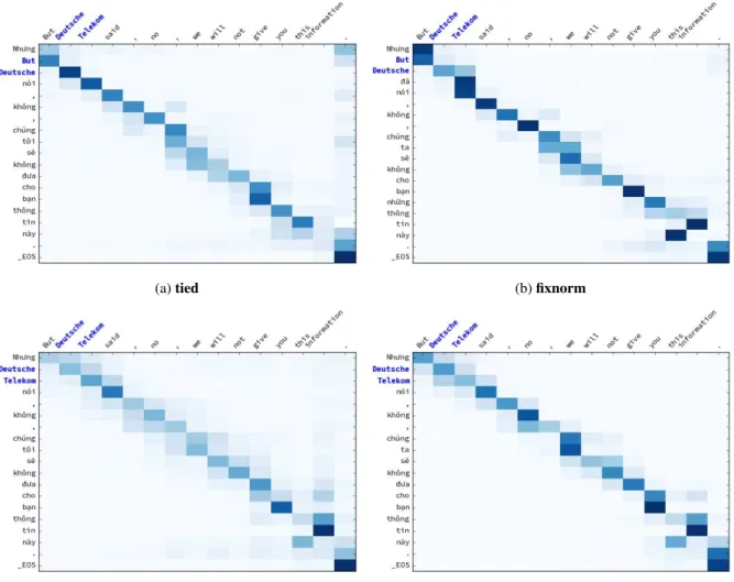
Both our baseline NMT andfixnormmodels suf-fer from the problem of shifted alignments noted by Koehn and Knowles (2017). As seen in Figure 2a and 2b, the alignments for those two systems seem to shift by one word to the left (on the source side). For example,nóishould be aligned tosaid
untied tied fixnorm fixnorm+lex Moses Arthur
ta-en 8.2 8.2 10.7 (+2.5) 12.5 (+4.3) 7.7 (−0.5)† 10.5 (+2.3) ur-en 6.1 8.4 10.1 (+1.7) 10.7 (+2.3) 11.8 (+3.4) 9.9 (+1.5) ha-en 11.6 12.9 15.1 (+2.2) 17.4 (+4.5) 17.2 (+4.3) 12.9 (+0.0)†
tu-en 7.3 8.7 11.8 (+3.1) 12.8 (+4.1) 11.0 (+2.3) 10.2 (+1.5) uz-en 9.8 8.8 11.7 (+2.9) 13.5 (+4.7) 10.4 (+1.6) 9.9 (+1.1) hu-en 14.8 14.5 16.7 (+2.2) 17.7 (+3.2) 13.7 (−0.8)† 15.2 (+0.7)†
en-vi 25.1 25.4 26.5 (+1.1) 26.7 (+1.3) 26.7 (+1.3) 25.9 (+0.5)† en-ja (BTEC) 51.2 52.8 54.0 (+1.2)† 51.7 (−1.1)† 46.8 (−6.0) 51.9 (−0.9)† en-ja (KFTT) 24.1 24.1 25.8 (+1.7) 26.2 (+2.1) 21.3 (−2.8) —
Table 3: Test BLEU of all models. Differences shown in parentheses are relative totied, with a dagger (†) indicating aninsignificant difference in BLEU (p > 0.01). While the method of Arthur et al. (2016) does not always help, fixnorm and fixnorm+lex consistently achieve significant improvements over tied(p<0.01) except for English-Japanese (BTEC). Our models also outperform the method of Arthur et al. on all tasks and outperform Moses on all tasks but Urdu-English and English-Vietnamese.
input Dushanba kuni Hindistonda kamida34kishi halok bo’lgani xabar qilindi .
reference At least34more deaths were reported Monday in India .
untied At leastUNKpeople have died in India on Monday .
tied It was reported that at least700people died in Monday .
fixnorm At least34people died in India on Monday .
fixnorm+lex At least34people have died in India on Monday .
input YarınKenya’dabir yardım konferansı düzenlenecek .
reference Tomorrow a conference for aid will be conducted inKenya.
untied Tomorrow there will be anAfghanrelief conference .
tied Tomorrow there will be a relief conference inMyanmar.
fixnorm Tomorrow it will be a aid conference inKenya.
fixnorm+lex Tomorrow there will be a relief conference inKenya.
input Ammo muammolar hali ko’p , deydi amerikalik olimEntoni Fauchi.
reference But still there are many problems , says American scientistAnthony Fauci.
untied But there is still a lot of problems , saysJames Chan.
tied However , there is still a lot of problems , says American scientists .
fixnorm But there is still a lot of problems , says American scientistUNK UNK.
fixnorm+lex But there are still problems , says American scientistAnthony Fauci.
Table 4: Example translations, in whichuntiedandtiedgenerate incorrect, but often semantically re-lated, words, butfixnormand/orfixnorm+lexgenerate the correct ones.
hu-en
244 244 (0.599) document (0.005) By (0.003) by (0.002) offices (0.001)
befektetéseinek investments (0.151) investment (0.017) Investments (0.015) all (0.012) investing (0.003) kutatás-fejlesztésre research (0.227) Research (0.040) Development (0.014) researchers (0.008) development (0.007)
tu-en
ifade expression (0.109) expressed (0.061) express (0.056) speech (0.024) expresses (0.020)
cumhurba¸skanı President (0.573) president (0.030) Republic (0.027) Vice (0.010) Abdullah (0.008)
Göstericiler protesters (0.115) demonstrators (0.050) Protesters (0.033)UNK(0.004) police (0.003)
ha-en
(0.469) cholera (0.003)EOS(0.001)UNK(0.001) It (0.001)
Wayoyin phones (0.414) wires (0.097) mobile (0.088) cellular (0.064) cell (0.061)
manzonsa Prophet (0.080) His (0.041) Messenger (0.015) prophet (0.010) his (0.009)
(a)tied (b)fixnorm
(c)fixnorm+lex (d) Arthur et al. (2016)
Figure 2: While thetied andfixnorm systems shift attention to the left one word (on the source side), ourfixnorm+lexmodel and that of Arthur et al. (2016) put it back to the correct position, improving unknown-word replacement for the wordsDeutsche Telekom. Columns are source (English) words and rows are target (Vietnamese) words. Bolded words are unknown.
0 10 20 30 40 50
0 5 10 15 20
epochs
BLEU
ha-en
tied fixnorm fixnorm+lex
0 10 20 30 40 50
0 10 20 30
epochs hu-en
tied fixnorm fixnorm+lex
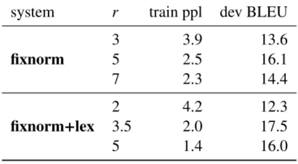
system r train ppl dev BLEU
fixnorm
3 3.9 13.6
5 2.5 16.1
7 2.3 14.4
fixnorm+lex
2 4.2 12.3
3.5 2.0 17.5
5 1.4 16.0
Table 6: Whenris too small, high train perplexity and low dev BLEU indicate underfitting; whenris too large, low train perplexity and low dev BLEU indicate overfitting.
6.4 Impact ofr
The single most important hyper-parameter in our models isr. Informally speaking, r controls how much surface area we have on the hypersphere to allocate to word embeddings. To better under-stand its impact, we look at the training perplex-ity and dev BLEUs during training with diff er-ent values ofr. Table 6 shows the train perplexity and best tokenized dev BLEU on Turkish-English for fixnorm andfixnorm+lex with different val-ues of r. As we can see, a smaller r results in worse training perplexity, indicating underfitting, whereas ifris too large, the model achieves better training perplexity but decrased dev BLEU, indi-cating overfitting.
6.5 Impact on training
One downside of our approaches is the need to project all word embeddings to the r-sphere, which is an expensive operation. Even though we only performed this operation after every ten updates, it still slowed down our training from roughly 2000 to roughly 1000 target words per second on English-Japanese (KFTT). On lower-resource settings, the impact was less, due to smaller vocabulary sizes.
We note that while both fixnorm and fixnorm+lex have a better initial start, they converge in roughly the same number of epochs as the baseline, as seen in Figure 3.
6.6 Lexicon
One byproduct of lex is the lexicon, which we can extract and examine simply by feeding each source word embedding to the FFNN module and calculatingpℓ(y)=softmax(Wℓhℓ+bℓ). In Table 5,
we show the top translations for some entries in the lexicons extracted fromfixnorm+lexfor Hun-garian, Turkish, and Hausa-English. As expected, the lexical distribution is sparse, with a few top translations accounting for the most probability mass.
7 Related Work
The closest work to ourlexmodel is that of Arthur et al. (2016), which we have discussed already in Section 4. Recent work by Liu et al. (2016) has a similar motivation to that of ourfixnorm model. They reformulate the output layer in terms of di-rections and magnitudes, as we do here. Whereas we have focused on the magnitudes, they focus on the directions, modifying the loss function to try to learn a classifier that separates the classes’ di-rections with something like a margin.
Handling rare words is an important problem for NMT that has been approached in various ways. Some have focused on reducing the num-ber of UNKs by enabling NMT to learn from a larger vocabulary (Jean et al., 2015; Mi et al., 2016); others have focused on replacingUNKs by copying source words (Gulcehre et al., 2016; Gu et al., 2016; Luong et al., 2015b). However, these methods only help with unknown words, not rare words. An approach that addresses both unknown and rare words is to use subword-level informa-tion (Sennrich et al., 2016; Chung et al., 2016; Luong and Manning, 2016). Our approach is dif-ferent in that we try to identify and address the root of the rare word problem. We expect that our models would benefit from more advanced UNK -replacement or subword-level techniques as well.
8 Conclusion
9 Acknowledgements
This research was supported in part by University of Southern California subcontract 67108176 un-der DARPA contract HR0011-15-C-0115. Nguyen was supported by a fellowship from the Vietnam Education Foundation. We would like to express our great appreciation to Sharon Hu for letting us use her group’s GPU cluster (supported by NSF award 1629914), and to NVIDIA corporation for the donation of a Titan X GPU. We also thank Tomer Levinboim for insightful discussions.
References
Philip Arthur, Graham Neubig, and Satoshi Nakamura. 2016. Incorporating discrete translation lexicons into neural machine translation. InProc. EMNLP.
Dzmitry Bahdanau, Kyunghyun Cho, and Yoshua Ben-gio. 2015. Neural machine translation by jointly learning to align and translate. InProc. ICLR.
Kyunghyun Cho, Bart van Merrienboer, Dzmitry Bah-danau, and Yoshua Bengio. 2014. On the properties of neural machine translation: Encoder-decoder ap-proaches. InProceedings of SSST-8, Eighth Work-shop on Syntax, Semantics and Structure in Statisti-cal Translation.
Junyoung Chung, Kyunghyun Cho, and Yoshua Ben-gio. 2016. A character-level decoder without ex-plicit segmentation for neural machine translation. InProc. ACL.
Jonas Gehring, Michael Auli, David Grangier, Denis Yarats, and Yann N. Dauphin. 2017. Convolutional sequence to sequence learning. arXiv:1705.03122.
Jiatao Gu, Zhengdong Lu, Hang Li, and Victor O.K. Li. 2016. Incorporating copying mechanism in sequence-to-sequence learning. InProc. ACL.
Caglar Gulcehre, Sungjin Ahn, Ramesh Nallapati, Bowen Zhou, and Yoshua Bengio. 2016. Pointing the unknown words. InProc. ACL.
Kaiming He, Xiangyu Zhang, Shaoqing Ren, and Jian Sun. 2016. Deep residual learning for image recog-nition. InProc. CVPR.
Hakan Inan, Khashayar Khosravi, and Richard Socher. 2017. Tying word vectors and word classifiers: A loss framework for language modeling. In Proc. ICLR.
Sébastien Jean, Kyunghyun Cho, Roland Memisevic, and Yoshua Bengio. 2015. On using very large tar-get vocabulary for neural machine translation. In Proc. ACL-IJCNLP.
Marcin Junczys-Dowmunt, Tomasz Dwojak, and Hieu Hoang. 2016. Is neural machine translation ready for deployment? A case study on 30 translation di-rections. InProc. IWSLT.
Philipp Koehn. 2004. Statistical significance tests for machine translation evaluation. InProc. EMNLP.
Philipp Koehn, Hieu Hoang, Alexandra Birch, Chris Callison-Burch, Marcello Federico, Nicola Bertoldi, Brooke Cowan, Wade Shen, Christine Moran, Richard Zens, et al. 2007. Moses: Open source toolkit for statistical machine translation. InProc. ACL.
Philipp Koehn and Rebecca Knowles. 2017. Six chal-lenges for neural machine translation. In Proc. Workshop on Neural Machine Translation.
Weiyang Liu, Yandong Wen, Zhiding Yu, and Meng Yang. 2016. Large-margin softmax loss for convo-lutional neural networks. InProc. ICML.
Minh-Thang Luong and Christopher D. Manning. 2015. Stanford neural machine translation systems for spoken language domain. InProc. IWSLT.
Minh-Thang Luong and Christopher D. Manning. 2016. Achieving open vocabulary neural machine translation with hybrid word-character models. In Proc. ACL.
Minh-Thang Luong, Hieu Pham, and Christopher D. Manning. 2015a. Effective approaches to attention-based neural machine translation. InProc. EMNLP.
Thang Luong, Ilya Sutskever, Quoc Le, Oriol Vinyals, and Wojciech Zaremba. 2015b. Addressing the rare word problem in neural machine translation. In Proc. ACL-IJCNLP.
Haitao Mi, Zhiguo Wang, and Abe Ittycheriah. 2016. Vocabulary manipulation for neural machine trans-lation. InProc. ACL.
Franz Josef Och and Hermann Ney. 2002. Discrimina-tive training and maximum entropy models for sta-tistical machine translation. InProc. ACL.
Franz Josef Och and Hermann Ney. 2003. A systematic comparison of various statistical alignment models. Computational Linguistics29(1).
Ofir Press and Lior Wolf. 2017. Using the output embedding to improve language models. In Proc. EACL.
Rico Sennrich, Barry Haddow, and Alexandra Birch. 2016. Neural machine translation of rare words with subword units. InProc. ACL.
Xing Wang, Zhengdong Lu, Zhaopeng Tu, Hang Li, Deyi Xiong, and Min Zhang. 2017. Neural machine translation advised by statistical machine transla-tion. InProc. AAAI.
Yonghui Wu, Mike Schuster, Zhifeng Chen, Quoc V Le, Mohammad Norouzi, Wolfgang Macherey, Maxim Krikun, Yuan Cao, Qin Gao, Klaus Macherey, et al. 2016. Google’s neural machine translation system: Bridging the gap between human and machine translation. arXiv:1609.08144.
Wojciech Zaremba, Ilya Sutskever, and Oriol Vinyals. 2014. Recurrent neural network regularization. arXiv:1409.2329.