Measuring and Analyzing Food
Intakes
Presented to NTU
2010.10.20
Hsing-Yi Chang
You are What you Eat
But do you who you are?
OUTLINE
Food and Nutrients
Measuring diet and their associated problems
Patterns vs. daily intakes
Examples
Validation of dietary measurements
Assess and cope in analysis with the errors which are likely to arise in dietary measurement
Nature of variation in diet
Estimation problems and corrections
References
Margetts, B.M. and Nelson, M. 2000, Design concepts in Nutri
tional Epidemiology
Willett, W. 1998, Nutritional Epidemiology
Nutrients vs. Foods
Representing diet as specific compounds or
groups of compounds
The information can be directly related to our
fundamental knowledge
The structure is known, ready to be synthesized
and used for supplementation
Total intakes is easy to use and powerful in
testing hypothesis
Nutrients vs. Foods
Analysis based on foods
Directly relate to dietary recommendations
Foods are an extremely complex mixture of
chemicals that may compete with, antagonize, or
alter the bioavailability of any single nutrient
contained in that food, it is not possible to predict
with certainty the health effects.
What Nutrition Epidemiologists Normally
Do After Collecting Data?
Compute the contribution of nutrient intake
from various food groups
Pattern analysis via factor analysis or
cluster analysis. Aggregate empirically
individuals with similar diets based on their
reported intake of foods.
Measuring diets/Intakes
Food Consumption
Commonly used methods for measuring nutrient
intakes
Chemical
analysis Food Composition Tables
Records Interview Short cut
Duplicate portio n
Aliquot samplin g
Equivalent com posite
Precise weighing Weighed inventory Intake record
Recall
Dietary history
Record Recall
Individual Surveys – 24 hr. Recall
Method for assessing present or recent diet
24-hour-recalls
Commonly used in cross-sectional studies
Interviewed or written information about the previous day’s intakes. Food items and quantities/portion sizes are recorded, if possible.
Advantages: quick and easy (NHANES III)
Subjects to day-to-day variation, miss-classification
• Repeated measurements are required to estimate the variation
The validity of the method has been assess by
comparing results with weighed records, diet histories, and biological markers. The results are not consistent.
Individual Surveys –24 hr. Recall
Dietary records
Subjects are taught to describe and give an
estimate of the weight of food immediately before
eating in writing or verbal records.
Normally, literate and highly motivated subjects would complete the task.
May alter eating behaviors while recording
Sources of errors
Respondent and recorder errors
Social desirability (obese subject under-report food or recording process alter eating behavior), forget to
record foods not eaten at home, etc.
Individual Surveys- Food Frequency
Food frequency questionnaire (FFQ)
Most frequently used. Assessing usual eating habits, over recent month or year.
Comprise a list of foods most informative about the
nutrients or foods of interests. Instruments vary from very short to a long list of over 100 food items.
Frequency and portion sizes should be closed rather than open. (This is to minimize coding errors). Always contain the options ‘never’.
Every questionnaire should be rigorously pre-tested and validated.
Approaches for Evaluating Dietary QN
Comparison of means with data from other
sources. This is done in the same population
Proportion of total intake accounted for by foods
included on the QN
Inclusion of 24-hr-recall for the important food
Compare the results from FFQ with 24-hr-recall
Reproducibility, repeated in few days or weeks
Validity: compare individual values with an independent measure of diet, say gold standard.
Compare with biochemical markers
Examples
NAHSIT
2009 NHIS
HALST
Food Composition Data Sources and
Computation
Exiting database: 食工所食物組成表
Extensive and comprehensive database for nutr
ient values of all foods that might be reported b
y subjects (for open questions like 24-hr-recall).
Computer software
Laboratory analysis
Nature of Variation in Diet
We are interested in long-term diet. An
understanding of day-to-day variation in dietary
intake is essential in choosing an appropriate
method to assess diet and to interpret data
collected by different approaches.
Source of variation
Day-to-day
Day of the week
Day of the season
Degree of variation differs according to nutrients
Macro nutrients, which contribute largely to caloric intake, are relatively stable
Micro nutrients, which tend to concentrate in certain foods, vary a lot.
Within Individual Variation
Between Individual Variation
Average of 194 women
Different Number of Days
Seasonal Variation
Estimating Within Individual Variation
Repeated Measures are needed
where ε represents day-to-day variation
The ratio of within to among individual variance (or
intra/inter variability) is
It can be estimated by where is the average
correlation coefficient between repeated
measurements.
2 2 b w
subjec
iNutrientY
1
( Liu et al, 1979)
ρ’s estimated by different studies
Effect of Within-individual-variation on
regression
Observed
True
2 2
2 2
2 2
)
|
var(
u x
x u
W
xY
0 xX cannot be observed, instead W is observed. W is the measurement with error, x is the true value.
W=X+U (Fuller 1987)
Effect of Within-individual Variation on
Association Studies
Correction for Attenuation
For the following situations
X is a scalar
The measurement error is additive with error variation estimated by
The covariates (X,Z,W) are jointly normally distributed
The response is affected by a linear combination of the p redictor, namely . This can be linear, log istic, probit of loglinear regression
For estimating the effect of X, namely β
x, the regr
ession calibration estimator is formed in three ste
ps
2
u
ˆ
u2
x
zt
0The Steps
Let be the naïve estimator formed by
ignoring measurement error
Let be the regression squared error for a
linear regression of W on Z. This is the sample
variance of the W’s if there are no other
covariates Z;
The regression calibration estimator is
ˆ
x2
ˆ
w|z
ˆ )
/( ˆ
) ˆ
Navive
ˆ (
2 2| 2
|z w z u
w
x
R. Carroll, D. Ruppert, and L.A. Stefanski, 1995
Estimating Population Distribution
Subject to within individual variations
Nusser et. Al, 1997, JASA
Transform data to normally distributed via Box-Co
x transformation
Estimate the within individual variation
Remove the within individual variation from the tot
al variance
Back transform the data to original scale based o
n normal with the new variance
Another Approach
Can be rewritten as
Estimation Steps
Estimate the within individual variance and the
ratio of within to among individual variance
Sampling weights
Estimate the parameters of the observed
distribution accounting for sampling weights
Estimate the adjusted variance by applying the
results of 1 to the results of 3
Reconstruct the adjusted distribution using the
results of 4
SAS program
Variation in 24-hr-recall (nutrients)
Ratio of Within to Among Variation
Nutrient 1% 25% 50% 75% 99% Energy (KCAL) 1662.1
(552.9) 1996.0 (1602.2) 2368.1 (2164.8) 2975.4
(2857.2) 4004.1 (8502.7) Protein (g) 52.2 ( 21.9) 78.2 ( 60.2) 90.9 ( 81.6) 105.4 ( 108.3) 145.7 ( 411.0) Fat (g) 39.7 ( 5.7) 66.7 ( 31.6) 80.7 ( 58.0) 97.0 ( 105.6) 145.4 ( 636.8) Carbohydrate
(g) 151.0 ( 49.0) 252.0 ( 213.2) 304.5 ( 292.3) 360.4 ( 370.4) 548.3 ( 814.3) Fiber (g) 1.7 ( 0.2) 3.8 ( 2.0) 5.0 ( 3.2) 6.5 ( 5.8) 11.2 ( 46.9) Calcium (mg) 220.7 ( 23.2) 382.2 ( 209.3) 467.9 ( 369.5) 564.0 ( 600.9) 851.4 (1951.0) Phosphorus
(mg) 630.9 (198.7) 1007.4
( 764.4) 1192.6 (1039.7) 1423.6
(1475.2) 2022.4 (5830.9) Iron (mg) 8.2 ( 1.7) 13.4 ( 8.4) 16.0 ( 11.9) 18.9 ( 18.7) 28.3 ( 117.7) Vitamin A (I. U.) 3251.7
( 80.5)
5630.0 (1533.3)
6843.7 (3188.7) 8260.3 (6885.6)
12932.0 (56173.6)
Vitamin B (mg) 0.8 ( 0.2) 1.2 ( 0.8) 1.5 ( 1.2) 1.7 ( 1.7) 2.5 ( 7.9) Vitamin B2 (mg) 0.7 ( 0.2) 1.2 ( 0.8) 1.4 ( 1.1) 1.7 ( 1.6) 2.4 ( 6.7) Niacin (mg) 9.4 ( 4.0) 15.7 ( 10.8) 19.0 ( 15.9) 23.0 ( 22.0) 34.5 ( 95.5) Vitamin C (mg) 47.2 ( 0.5) 119.5 ( 42.6) 161.9 ( 92.3) 214.7 ( 175.0) 400.0 (1425.9) SFA (g) 11.8 ( 1.7) 21.9 ( 10.4) 27.1 ( 17.9) 33.3 ( 34.9) 52.6 ( 218.5) PFA (g) 11.4 ( 1.0) 17.5 ( 7.8) 21.2 ( 14.4) 24.2 ( 28.1) 34.0 ( 110.0) Oleic acid (g) 11.9 ( 1.9) 23.7 ( 11.4) 30.3 ( 19.6) 37.6 ( 39.6) 61.3 ( 281.6) Cholesterol
(mg) 169.2 ( 3.7) 330.8 ( 175.1) 417.1 ( 393.8) 521.5 ( 620.9) 837.8 (1240.0)
Problem With Large Number of 0’s
There are two kinds of zero’s in the 24 hr. recall
data.
One is that the individual never eats the food.
The other is the individual did not eat the food 24 hours before the interview
.
The Food Frequency Questionnaire provides
information on whether an individual consume
certain food.
We used this information to identify which kind of zero is observed in 24-hr-recall
Method
We use the Zero-Inflated Model to model usual food
intakes with large number of zero’s. The distribution
function of the amount of usual food intakes is
following:
if F x 1 p pF
a x
x 0
Otherwise F 0 1 p
is a random variable that represents the amount of
usual intake for some kind of food
is the probability that an individual consume this food
x
p
Correction for the effects of measurement error
In estimating the usual intakes, the first task is to estimate the ratio of within-to-amon g variation. We use the method proposed by Delcourt (1994) that estimate the correl ation coefficient of the amount of intakes measured at two time point firstly.
Consider that the Pearson correlation coefficient can be expressed as:
Suppose that there are two time point measures. and are the standard deviati on for the first time measure and the second time measure. is the estimation of Pe arson correlation coefficient between measures.
Let is used to estimate . Then ,
is a modified estimate of .
When there are more than two time points, the average coefficient is used.
2 2
2 e s
s
s
2
12 22
22 s s
s
s2
e2
2
sr
r
s
2s
1
x pf
xf
a x 0
f
aThe density function is when
If
follow a gamma distribution with parameter α, β
x
a
x x e
f
1
1The overall mean is pαβ, and the variance is
p
2αβ
2.
Example
估計米飯類的飲食量分配
G1 米類:
G1_1 米類:糙米、糯米、胚芽米、小米等。
G1_2 加工製品類:新竹米粉、米糕、米漿等。
Example (data)
24-Hour Dietary Recall
已經整理好的資料檔,欄位包含有性別、地區層
別、問卷權數、年齡、 G1~G27(27 種食物類別 )
和個案編號。
Example (data)
重覆測量資料
欄位有性別、問卷權數、重覆個案編號、年齡、
G1~G27(27 種食物取用量 )
Example (data)
Food-Frequency Questionnaires (FFQ)
欄位包含有
Example (sas code)
資料整理
截取米飯類食用量 (24-Hour Dietary Recall) data food_G1; /* 製作一個新的檔案 */
set Tmp1.Big;
if G1=0 then delete; /* 當食用量不為 0 的時後 , 選入檔案 */ keep id agecate order sex stra agen qwt G1;
run;
截取米飯類食用量 ( 重覆測量資料 )
data food_R_G1; set Tmp1.Rv_Big; if G1=0 then delete;
keep id agecate order sex stra agen qwt G1; run;
合倂檔案
proc sort data=food_G1; by id;
proc sort data=food_R_G1 by id;
run; data G1;
merge Food_g1 Food_r_g1; by id ;
if G1 and H1; run;
Example (sas code)
計算參數估計值
proc corr data=G1; var G1 H1;
run; Simple Statistics
Variable N Mean Std Dev Sum Minimum Maximum G1 534 139.46474 115.96585 74474 0.06940 1127 H1 534 126.63431 97.76724 67623 1.55232 643.85882
Pearson Correlation Coefficients, N = 534 Prob > |r| under H0: Rho=0 G1 H1 G1 1.00000 0.31677 <.0001 H1 0.31677 1.00000 <.0001
S1 S2 γ α*β α*β^2 α β
115.96 97.77 0.32 133.05 3680.91 4.81 27.67
Example (sas code)
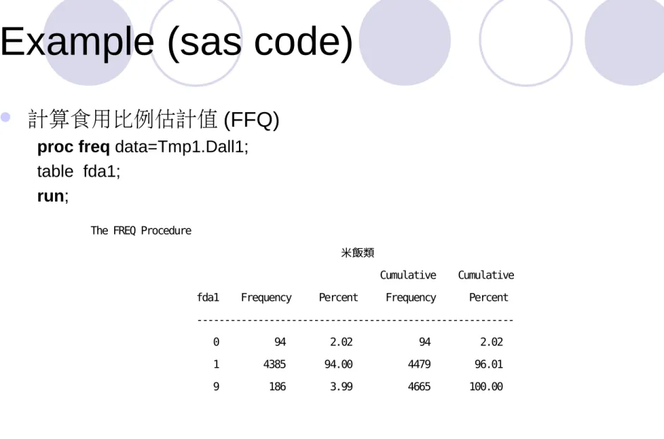
計算食用比例估計值 (FFQ)
proc freq data=Tmp1.Dall1; table fda1;
run;
96.01/(96.01+2.02)=0.98
The FREQ Procedure
米飯類
Cumulative Cumulative fda1 Frequency Percent Frequency Percent --- 0 94 2.02 94 2.02 1 4385 94.00 4479 96.01 9 186 3.99 4665 100.00
Example (estimation of the distribution)
利用 Excel 函數 GAMMAINV(probability,alpha,b
eta) 畫出食用量的分配圖形
相關參數