本文 総合研究大学院大学学術情報リポジトリ 甲1482 本文

Interaction between Static Magnetic Islands

and Interchange Modes in Heliotron Plasmas

Kinya Saito

DOCTOR OF PHILOSOPHY

Department of Fusion Science

School of Physical Science

The Graduate University for Advanced Studies

2011

Abstract

Nonlinear interaction between static magnetic islands generated by an external field and a resistive interchange mode driven by pressure gradient is investigated in straight heliotron configurations by means of a numerical method based on the reduced mag- netohydrodynamics (MHD) equations. For the comprehensive understanding of the interaction, two aspects are studied by utilizing different MHD equilibria. One is ef- fects of the interchange mode on the change of the static island and the other is effects of the static island on the growth of the interchange mode.

Firstly, the former interaction aspect is studied with an equilibrium corresponding to nested magnetic surfaces. In this case, the interchange mode grows in spite of existence of a static magnetic island. The island width is changed in the nonlinear saturation phase of the interchange mode. The situation of the increase or decrease of the width depends on whether the diffusion of the equilibrium pressure in the direction parallel to the magnetic field is taken into account or not. In the case without the effect of the diffusion of the equilibrium pressure, there exist two solutions corresponding to the increase and the decrease of the island width. In this case, in spite of the nonlinear interaction, the total poloidal flux is approximately given by the linear sum of the poloidal flux generated by the interchange mode without a static island and the external poloidal flux for the generation of the static island. In the case with the effect of the diffusion of the equilibrium pressure, there exists only one solution corresponding to the increase of the width. This is due to the fact the parallel diffusion term generates a pressure term corresponding to the increase of the island width.

Next, the latter interaction aspect is studied. For this study, equilibria including static magnetic islands are necessary because the equilibrium pressure profile consistent with the magnetic islands has possibility to affect the stability of the interchange mode. We have developed a numerical code (FLEC) to calculate the equilibria and found that there exist two kinds of solutions. One is the equilibrium of which the pressure profile is flat at not only the O-point but also the X-point. In this case, the pressure gradient

i

is continuous at the separatrix. The other is the equilibrium of which the pressure profile is flat at the O-point and steep at the X-point. In this case, the pressure gradient is discontinuous at the separatrix of the magnetic island. The finite beta has a contribution to increase the island width.

Since it is known that the pressure profile with annular local flat structure around the resonant surface have a stabilizing contribution to the interchange mode, effects of the static island on the interchange mode is studied for the equilibrium with the steep gradient at the X-point. The linear growth rate of the interchange mode is decreased and the saturation level is reduced as the island width is increased. The mode is completely stabilized when the width exceeds threshold value. In the case that interchange modes are unstable in an equilibrium with a thin island width, there are two cases of the increase and the decrease of the island width in the nonlinear saturation of interchange modes as obtained in the study for the former interaction aspect.

Acknowledgements

First of all, I would like to thank Professor Katsuji Ichiguchi, who gave me the op- portunity to study the plasma physics, fruitful guidance and warm encouragement throughout my doctoral course. I would also like to acknowledge Dr. Ryuichi Ishizaki for his valuable suggestion. This thesis is based on the discussion with them.

I would like to thank Dr. Yasuhiro Suzuki (NIFS) and Dr. Ryutaro Kanno (NIFS). They gave me useful suggestions and lots of comments for numerical calculation of magnetohydrodynamics equilibria including a static magnetic island. I also thank Emeritus Professor Nobuyoshi Ohyabu for his guidance.

I would also like to extend my appreciation to Professor Kiyomasa Watanabe (NIFS) and Dr. Satoru Sakakibara (NIFS). They provided me the LHD experimental data and allowed me to use the experimental data for my presentation.

I express my gratitude for Dr. Yoshiro Narushima (NIFS) and Dr. Shinichiro Toda (NIFS). A seminar with them helped me establish a firm foundation for ideal magnetohydrodynamics.

I would also like to acknowledge Professor Hideo Sugama (NIFS), Dr. Masaru Furukawa (Tokyo Univ.) and Professor Fumimichi Sano (Kyoto Univ.) for a lot of suggestions.

Dr. Seikichi Matsuoka (NIFS), Dr. Motoki Nakata (JAEA), Dr. Kunihiro Ogawa (Nagoya Univ.), Mr. Kohki Kumagai (IHI), Dr. Seiya Nishimura (NIFS) and Dr. Ryousuke Seki (NIFS) are acknowledged for their advise and suggestions of my the- sis. Furthermore, I thank Dr. (to be) Akiyoshi Murakami (Sokendai), Dr. (to be) Shinya Maeyama (Tokyo Tech.) and Mr. Masahito Naito (SANSHODO) for their encouragement.

Finally, I would like to express my acknowledgments to my parents; Yoshikazu Saito and Chizuko Saito. They support me all the time.

iii

Contents

Abstract i

Acknowledgements iii

1 Introduction 1

2 Model Equations and Expression of Static Magnetic Islands 7 2.1 Reduced MHD equations . . . 7 2.2 External poloidal flux . . . 10 3 Effects of Interchange modes on Behavior of Static Magnetic Islands 13 3.1 Introduction . . . 13 3.2 Change of magnetic island in nonlinear evolution of interchange modes 14 3.2.1 Equilibrium and linear analysis . . . 14 3.2.2 Behavior of interchange mode without static magnetic islands 15 3.2.3 Interaction between static magnetic island and interchange mode 19 3.2.4 Discussion . . . 37 3.3 Effect of parallel diffusion of equilibrium pressure on island behavior . . 40 3.3.1 Island evolution due to interchange mode . . . 40 3.3.2 Mechanism of increase in island width . . . 45 3.4 Summary . . . 47

4 MHD Equilibria including Static Magnetic Islands 51

4.1 Introduction . . . 51 4.2 Coupled equations for equilibrium calculation . . . 53 4.3 Equilibrium calculation utilizing diffusion equation parallel to the field

line . . . 54 4.3.1 Numerical method . . . 54

v

4.3.2 Resultant equilibrium . . . 58

4.3.3 Pressure profile with perpendicular heat conductivity . . . 62

4.4 Method by tracing field line . . . 72

4.4.1 Averaged pressure along the field line . . . 72

4.4.2 Calculation procedure with field line tracing method . . . 74

4.4.3 Resultant equilibrium . . . 75

4.5 Discussions . . . 76

4.6 Summary . . . 77

5 Stability of Interchange Modes in Equilibrium including Static Island 85 5.1 Introduction . . . 85

5.2 Island effect on linear stability . . . 86

5.3 Nonlinear interaction between static magnetic islands and interchange modes . . . 89

5.4 Summary . . . 91

6 Conclusions 101

A Improvement of the NORM code 105

B Development of the FLEC code 109

Bibliography 114

List of Publication 119

Chapter 1

Introduction

In magnetic confinement of fusion plasmas, existence of nested magnetic surfaces is desirable for the good confinement. However, error magnetic fields originated from misalignment of field coils and the terrestrial magnetism induce static magnetic is- lands. The static islands have a possibility to degrade the plasma confinement sub- stantially. Therefore, it is one of the essential themes in magnetic confinement systems to understand how such islands grow or decay in finite beta plasmas. Hence, such island behavior has been studied extensively in both tokamaks and heliotrons [1]. In tokamaks, a lot of efforts are paid for the control of the edge localized mode with the island generation by the application of resonant magnetic perturbations (RMP) [2]. In heliotrons, the growth and the decay of the static magnetic islands at finite beta are studied. Particularly, in the large helical device (LHD) [3], which is the largest he- liotron device, the local island divertor (LID) coils are installed in the system [4]. The RMP or the error field can be generated actively by the currents in the LID coils and utilized for the study of the static islands behavior. The static magnetic islands are generated by the error field mainly with (m, n)=(1,1) and they affect plasma confine- ment and magnetohydrodynamics (MHD) properties. Here m and n are the poloidal and toroidal mode numbers, respectively. Spontaneous change in the islands and the influence on the confinement are analyzed in the experiments by controlling the static islands. Ohyabu et al. [5] studied the beta dependence of the self-healing of the islands. They found that the onset beta value of the self-healing is increased and nearly pro- portional to the externally imposed resonant error field. Narushima et al. [6] examined the dependence of the self-healing on the beta and the collisionality. They also showed that the sign of the perturbed magnetic field reversed suddenly when the beta exceeded the critical value of the self-healing.

1

The magnetic islands can also be generated by resistive MHD instabilities. In the heliotron configurations such as LHD, a net toroidal current is not needed for the generation of the confinement field. Therefore, tearing modes are not excited except a special case where a net toroidal current with a quite peaked profile flows in the plasma [7]. Instead, a magnetic hill usually exists in the plasma confinement region. Therefore, a resistive interchange mode driven by a pressure gradient can be excited in the configurations. Since the interchange modes can cause a collapse of the plasma [8], the stability control is important for a good confinement at high beta.

Thus, the interchange modes are the crucial MHD modes in the heliotron config- urations, and therefore, a lot of theoretical analyses have been done for the behavior. Particularly, Ichiguchi et al. and Ishizawa et al. [9–11] showed that magnetic islands are generated by nonlinear saturation of interchange modes numerically. Therefore, it is expected that the change of the static island width is caused by the interchange modes. On the other hand, magnetic islands have a potential to affect the stability of interchange modes. That is, the magnetic islands and the interchange modes can interact with each other.

However, comprehensive theoretical study about the direct interaction between the interchange mode and the static islands has not been carried out. Only a few works treated the dynamics of the interchange mode in the existence of the static islands. Unemura et al. [12] discussed the variation in the island width and the pressure profile due to the nonlinear evolution of the interchange mode in a straight heliotron con- figuration. However, they used multi-helicity perturbations and evaluated the island width in transitional regions of the time evolution. Garcia et al. [13, 14] also studied the nonlinear coupling of a static magnetic island and the interchange mode. In the studies, the diamagnetic effect is involved to investigate the shear flow effect. Because of the diamagnetic flow, the island width is oscillating even in the saturation state of the interchange mode. Therefore, the fundamental mechanism in the interaction of the islands and the interchange mode is difficult to be understood from these previous works.

Thus, we analyze the fundamental interaction between the static magnetic islands and the dynamics of the interchange mode numerically based on the reduced MHD equations [15]. A straight LHD configuration is employed as the magnetic configu- ration to see the interaction clearly. In order to investigate the fundamental interac- tion, we focus on the interaction between the static islands with the mode number of (m, n)=(1,1) and the interchange mode with the same mode number.

Two aspects of the interaction are studied. One is the effect of the interchange mode on the change of the static island and the other is the effect of the existence of the static island on the growth of the interchange mode. We examine these aspects separately by employing two procedures with different pressure profiles.

For the analysis of the former aspect, a pressure profile corresponding to a nested magnetic surface is employed. In this case, we obtain an equilibrium with the pressure profile which is unstable for the interchange mode, firstly. Therefore, effects of the static island on the equilibrium quantities are not included. Then, both of an error field generating a static island and the perturbation of the interchange mode are imposed simultaneously. Since there exists a finite pressure gradient inside the separatrix of the island, the interchange mode grows. In the growth, the interchange mode interacts with the static island nonlinearly. We follow the nonlinear evolution of the mode and evaluate the change of the island in the saturation phase of the nonlinear evolution. This procedure is suitable for the study of the effect of the interchange mode on the static island because the growth of the mode is guaranteed. This procedure is also employed in the studies of Ref. [12–14].

For the analysis of the latter aspect, we employ a pressure profile corresponding to the island geometry. When the beta value is increased gradually from the vacuum magnetic surfaces without the self-healing of the island, an equilibrium is achieved with a pressure profile of which the gradient inside the separatrix is reduced. In the equilibrium, the growth of the interchange mode is affected by the pressure profile. In order to study the island effect on the mode, we develop a numerical code to calculate such an equilibrium with the pressure profile corresponding to the island geometry. Since the behavior of the interchange mode is examined with the reduced MHD equa- tions, the equilibrium equations have to correspond to the reduced MHD equations, and therefore, they are coupled equations for the pressure and the poloidal magnetic flux.

The development of numerical codes to solve an equilibrium including magnetic islands has a long history. The pioneering work is the code developed by Chodura and Schl¨uter [16]. In this code, an equilibrium is obtained by minimizing the potential energy with a friction method on cylindrical coordinates based on the variational prin- ciple. Hender et al. developed the NEAR code by improving the Chodura-Schl¨uter code with the employment of vacuum flux surfaces for the reference coordinates [17]. Recently, the PIES code [18] and the HINT code [19, 20] or the HINT2 code [21] have been developed and widely used for the stellarator equilibrium studies. Both codes are

3

based on an iteration scheme of two steps. In the first step, the pressure profile con- sistent with the magnetic geometry with the magnetic field fixed. In the second step, the magnetic field satisfying the force balance equation is obtained with the pressure fixed. In the present work, we basically employ the two-step scheme.

The treatment in each step is different between the PIES and the HINT codes. In the first step of the PIES code, the pressure satisfying the equation of B · ∇P = 0 for a given magnetic field B is obtained with the field line tracing. In the second step, the plasma current is calculated by using this pressure P and the field is obtained by solving the Amp´ere’s law directly. Then, quasi magnetic coordinates are constructed with the field, and the next iteration is operated on the coordinates. The HINT code is based on the numerical scheme which was developed by Park et al. [19] for the reduced MHD equations, and is extended to the full MHD equations. Especially, the coordinate system twisted along the toroidal direction is employed for saving calculation regions. In the first step, the pressure satisfying B · ∇P = 0 is obtained as in the PIES code. The code by Park et al. and the original HINT code solve the equation by making the magnetic sound wave decay. The HINT2 code is improved so as to solve the equation B· ∇P = 0 directly by tracing the field lines. In the second step, a relaxation precess of the field is conducted with the equation of motion and the Faraday’s law with P fixed for obtaining the magnetic field satisfying the force balance condition.

In the present study for the latter effect, two kinds of numerical approach are employed in developing the equilibrium code. Both of them are based on the two- step scheme employed in the code by Park et al. and the HINT code, however, the numerical approach in each step is different. One is the combination of a diffusion equation for the pressure and an ordinary equation for the force balance. The other is the combination of a field line tracing method for the pressure and a relaxation method. The equilibrium solutions are different depending on the approach, particularly in the structure of the pressure profile.

By utilizing the equilibrium solutions, we examine the dependence of the linear stability and the nonlinear saturation of the interchange mode on the island width. Particularly, we focus on the effect of the existence of the finite pressure gradient at the X-point, because the interchange mode is driven by the pressure gradient. The stabilization effect of the annular flat structure of the pressure profile was analyzed by Ichiguchi et al. [22, 23]. However, the effect of the local flat structure with a finite gradient at the X-point has not been examined. Thus, we study the dependence of the linear growth rate and the saturation level on the island width by utilizing the

equilibrium with such structure. We also analyze the effect of the nonlinear saturation of the interchange mode on the change of the island structure as well.

The framework of this thesis is shown in Fig.1.1. In Chapter 2, the reduced MHD equations used in the analysis of the interchange mode dynamics and the introduction of the static island are explained. In Chapter 3, the results of the effect of the interchange mode on the change of the static island with the pressure profile corresponding to the nested magnetic surfaces are shown. We mainly focus on the changes of the width and the phase of the island in the saturation of the interchange mode. We also show the dependence of the island change on the effect of the equilibrium pressure diffusion in the parallel direction of the field line and discuss the mechanism of the island behavior. In Chapter 4, the equilibrium calculation including the static island is discussed. The two approaches of the equilibrium calculation are explained. The obtained solutions are compared with each other and the reason of the difference is discussed. In Chapter 5, the effect of the existence of the static island in the equilibrium on the behavior of the interchange mode is studied. We discuss the dependence of the linear stability and the nonlinear saturation level. In Chapter 6, conclusions are given.

5

Chapter 2

Chapter 3

MHD equilibrium corresponding to nested magnetic surfaces

Stability of interchange modes with static magnetic islands

・case with parallel diffusion

・case without parallel diffusion

Chapter 4

Stability of interchange modes in equilibrium including static island Chapter 5

Conclusions Chapter 6 Chapter 1 Introduction

Model equations and expression of static magnetic islands

MHD equilibria including static magnetic islands

Figure 1.1: Framework of this thesis.

Chapter 2

Model Equations and Expression of

Static Magnetic Islands

2.1 Reduced MHD equations

We study the interaction between the static islands and the interchange mode with (m, n)=(1,1). For the behavior of the plasma with such low mode numbers, the toroidally averaged field line curvature plays a dominant role. Therefore, the reduced MHD equations [15] are useful for this analysis, which are the equations for poloidal magnetic flux Ψ, stream function Φ and plasma pressure P . In a straight heliotron configuration, the normalized reduced MHD equations with the cylindrical coordinates (r,θ,z) are given by the Ohm’s law,

∂Ψ

∂t = −B · ∇Φ + _S^{1Jz, (2.1)}

the vorticity equation, dU

dt ^{= −B · ∇Jz+} 1

2ǫ²∇Ω × ∇P · z + ν∇²⊥^{U (2.2)}

and the plasma pressure equation, dP

dt ^{= κ⊥∇}

2⊥^{P + κ}k(B · ∇)(B · ∇)P. ^(2.3) The magnetic field B(r, θ, z) is expressed as

B(r, θ, z) = z + z × ∇Ψ(r, θ, z), ^(2.4) where z denotes the unit vector in the z direction. Here Jz, U and ∇Ω denote the current density in the z direction, the vorticity in the negative z direction and the

7

averaged magnetic field line curvature, respectively. The convective time derivative is given by

d dt ⁼

∂

∂t^{+ v⊥· ∇. (2.5)}

Here the velocity v⊥ is given by

v_{⊥= ∇⊥Φ × z, (2.6)}

where the operator ∇^⊥ is defined as

∇^⊥ = ∇ − z^{µ ∂}_∂z

¶

. (2.7)

The resistivity, the viscosity, the perpendicular and parallel heat conductivities are introduced with the coefficients of S, ν, κ⊥ and κk, respectively. Here, S denotes the magnetic Reynolds number expressed as

S = τR/τA, (2.8)

where the Alfv´en time τA and the resistive diffusion time τR are given by τA = R0^√µ0ρ/B0 and τR = µ0a²/η, respectively. The quantities R0, µ0, ρ, B0, a, η and ǫ denote the major radius of the corresponding torus, the vacuum permeability, the mass density, the magnetic field at the magnetic axis, the plasma radius, the resis- tivity and the inverse aspect ratio, respectively. In this study, we employ ǫ = 0.16, which corresponds to the LHD plasma. The quantities (r, z, t, Ψ, Φ, P, U, Jz, ν, κ_⊥, κ_k) are normalized by (a, R0 , τA, a²B0/R0, a²/τA, B₀²/2µ0, 1/τA, B0/µ0R0, ρa²/τA, a²/τA, R₀²/τA), respectively.

We analyze the interaction by tracing the time evolution of the interchange mode with the NORM code [9] numerically. The original NORM code solves the reduced MHD equations without the effect of the static islands. The equations are formulated in the time evolution form of the perturbed variables in the following way:

∂ ˜Ψ

∂t ^{= −B · ∇˜Φ +} 1

S^{J˜z, (2.9)}

d ˜U

dt = −(B · ∇ ˜^{Jz+ ˜B}· ∇J^{z eq) +} _2ǫ¹₂∇Ω^eq× ∇ ˜P · z + ν∇²⊥^{U˜ (2.10)}

and

d ˜P

dt ^{= (z × ∇˜Φ) · ∇Peq+ κ⊥∇}

2

⊥^{P + κ˜ k}(B · ∇)(B · ∇) ˜^{P . (2.11)}

The subscript of

is employed. Here, σ denotes the sign taking the value of +1 or -1 and f (r) should be a small and arbitrary function except eigenfunctions. In this study, the function of

f (r) = 10⁻¹⁶ⁿ_{1 − 4} µ

r − ¹₂

¶2

o2

(2.20) is used.

We monitor the time evolution of the these quantities to know how the mode grows. For this purpose, the kinetic energy EK and the magnetic energy EM are calculated, where EK and EM are given by

EK =

Npe

X

n=0,m=n

E_K^m,n, E_K^m,n = ¹ 2

Z

|∇^⊥Φm,nsin(mθ − nz)|^{2dV (2.21)}

and

EM =

Npe

X

n=0,m=n

E_M^m,n, E_M^m,n = ¹ 2

Z

|∇^⊥Ψm,ncos(mθ − nz)|^{2dV, (2.22)} respectively. Here,R dV denotes the integral over the plasma volume. The growth rate of the interchange mode γ is calculated from EK as

γ = ¹ 2

1 EK

dEK

dt ^{. (2.23)}

2.2 External poloidal flux

The static island generated by an error field is incorporated by assuming that the (m, n)=(1,1) component of the poloidal flux has a finite value at the boundary, r = 1. Here, we introduce an external poloidal flux Ψ^ext_m,n given by

Ψ^ext_m,n(r, θ, z) = ˆΨ^ext_m,n(r) cos(mθ − nz). ^(2.24) Since the external poloidal flux Ψ^ext_m,n does not induce any current density, Ψ^ext_m,n satisfies the equation

∇²⊥^Ψextm,n ^{= 0 (2.25)}

with the boundary conditions,

Ψˆ^ext_m,n(r = 0) = 0 (2.26)

and

Ψˆ^ext_m,n(r = 1) = Ψb = constant. (2.27)

Figure 2.1: Magnetic surfaces for Ψb _{= +2.0×10}⁻³. Blue line indicates the separatrix of the island. The island width is 1.01 × 10⁻¹ normalized by plasma radius.

Here, Ψb denotes the external poloidal flux at r = 1. Substituting Eqs.(2.15) and (2.24) to Eq.(2.25), Eq.(2.25) becomes

d²Ψ^ˆext_m,n dr^{2 +}

1 r

d ˆΨ^ext_m,n dr ⁻

m² r^{2 Ψˆ}

ext

m,n ^{= 0. (2.28)}

The solution of Eq.(2.28) is the linear combination of r^m and r^−m. In the case of (m, n) = (1, 1), Ψ^ext_1,1(r) is given by

Ψ^ext_1,1 = ˆΨ^ext_1,1(r) cos(θ − z), ^Ψˆext1,1^{(r) = Ψbr. (2.29)}

Figure 2.1 shows magnetic surfaces for Ψb = +2.0 × 10⁻³. Blue line indicates the separatrix of the island. The island width is 1.01 × 10⁻¹ normalized by plasma radius. The static island width can be controlled by changing the value of Ψb.

11

Chapter 3

Effects of Interchange modes on

Behavior of Static Magnetic Islands

3.1 Introduction

The effect of the interchange modes on the change of the static islands is studied in this Chapter. In order to understand the effect clearly, we assume an MHD equilibrium having nested magnetic surfaces firstly, then we impose the static island and perturba- tions of the interchange mode. We obtain the equilibrium quantities by averaging the three-dimensional equilibrium quantities based on the modified stellarator expansion method [24]. Such a treatment of the static island is also utilized in Ref. [12–14]. This situation may be close to the experiment by Sakakibara et al. [25]. They observed a collapse in the profile of the electron temperature (Te). The Te profile had a finite gradient at the

´

ι = 1 surface before the collapse in spite of that a natural error field with (m, n) = (1, 1) existed, where

´

ι indicates the rotational transform. The formation of local flat structure is observed in the Te profile during the collapse at the

´

^{ι = 1}

surface. This observation may indicate the static island appeared when an instability occurred.

We focus on the change of the island width and the island phase after the nonlinear saturation of the interchange mode. For this purpose, we trace the nonlinear time evolution of the interchange mode by using the NORM code. The mechanism of the changes in the island by the nonlinear saturation is discussed. As a general property of the interchange mode, the linear growth rate is increased with the mode number in the case without the dissipation effects of viscosity and heat conductivity. Inclusion

13

of the dissipations reduces the growth rate the more effectively for the higher mode number. Since we study the interaction between the interchange mode and the static island with the mode number of (m, n) = (1, 1), we choose appropriate coefficients of the dissipations so that the (m, n)=(1,1) mode has the largest growth rate in the single helicity perturbations.

We also study the effect of the heat conductivity for the equilibrium pressure in the direction parallel to the magnetic field. This conductivity gives a qualitative difference to the island behavior because the conductivity term is an inhomogeneous term in the reduced MHD equations. This term generates an initial perturbation of the interchange mode.

This chapter is organized as follows. In Section 3.2, the equilibrium and the linear analysis are described, and then, the change of the magnetic island in the nonlinear evolution of the interchange mode is discussed. In Section 3.3, the effect of parallel heat conductivity for equilibrium pressure on the island behavior is analyzed. In Section 3.4, a summary is given.

3.2 Change of magnetic island in nonlinear evolu-

tion of interchange modes

3.2.1 Equilibrium and linear analysis

We use a straight heliotron equilibrium corresponding to the LHD configuration with the vacuum magnetic axis located at 3.6m. The equilibrium is constructed by utilizing a three-dimensional equilibrium, which is calculated with the VMEC code [26] under the no net toroidal current and the free boundary conditions. We employ the equilibrium pressure profile given by

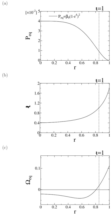
Peq= β0_{(1 − r}⁴)². (3.1)

Here, the beta value at the axis of β0 = 4.0% is employed. Figure 3.1 shows the profiles of Peq,

´

^{ι and Ωeq}. The profile of Ωeq is given by [24]

Ωeq(r) = ¹ 4π²

Z 2π 0

dθ Z 2π

0

dζ^{µ R} R0

¶2^Ã

1 + ^|B

3Deq − B^3Deq |² B²₀

!

, (3.2)

where ζ and R are the toroidal angle and the major radius, respectively. Here, B^3D_eq denotes the three-dimensional equilibrium field. The bar denotes the quantity averaged

toroidally over a field period. Dashed lines show the position of the rational surface with

´

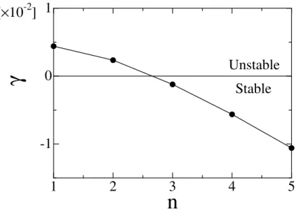
ι = 1. The surface is located at r = 0.85 where a substantial pressure gradient exists. The gradient of Ωeq is positive at the surface, which corresponds to a bad curvature of the field line and indicates a potential to drive a resistive interchange mode.

For the study of the interaction with the (m, n)=(1,1) island, the (m, n)=(1,1) component in the interchange mode has to be dominant in the nonlinear state. In order to obtain this situation, we determine the dissipation parameters of ν, κ⊥ and κk so that the component of (m, n)=(1,1) has the largest linear growth rate. We also employ a high resistivity to enhance the effect of the interchange mode. The NORM code is also utilized for the linear analysis. As the initial perturbations, Eq.(2.19) is employed. As the result of the linear mode analysis, the parameters of

S = 10⁴, ν = 8.0 × 10^{−5, κ}⊥^{= 10−5, κ}k ^{= 1.0 (3.3)}

are found to be suitable for the present analysis. Figure 3.2 shows the dependence of γ given by Eq.(2.23) on n for Ψb = 0 and σ = +1. Only the n = 1 and n = 2 modes are unstable, and the others are stable. The growth rate of the n = 1 mode is 1.9 times larger than that of the n = 2 mode. Figure 3.3 shows the linear eigenfunctions of the n = 1 mode. The poloidal flux ˆΨ_1,1 is a nearly odd function with respect to the resonant surface of

´

ι = 1. The stream function ˆΦ1,1 and the pressure ˆP1,1 are nearly even functions, both of which are localized around the resonant surface. These eigenfunctions show typical mode structures of the resistive interchange mode. In the change of σ, the sign of the eigenfunctions is opposite and the growth rate is unchanged because they are linear solutions.

3.2.2 Behavior of interchange mode without static magnetic

islands

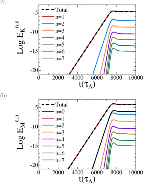
Before the discussion of the case with the static islands, we examine the dynamics of interchange modes under no static island. In the study of this Section, Eqs.(2.9)-(2.11) are utilized. Figure 3.4 shows the nonlinear time evolution of the kinetic energy and the magnetic energy for Ψb = 0 and σ = +1.

After the linear growth(t & 8500τA), a steady state appears. The n = 1 component is dominant in the steady state. Figure 3.5 shows the mode structure of the n = 1 component at t = 10000τA. The structure is similar to that of the linear eigenfunctions

15

(a)

0 0.2 0.4 0.6 0.8 1

0 1 2 3 4 [×10^-2]5

r

P

eq

ι=1

P_eq=_β0(1-r⁴)²

-

(b)

0 0.2 0.4 0.6 0.8 1

0 0.4 0.8 1.2 1.6

2

^ι=1

r

ι

-

(c)

0 0.2 0.4 0.6 0.8 1

0 0.1

r

Ω

eq

ι=1 ^-

Figure 3.1: Profiles of (a) pressure, (b) rotational transform and (c) average field line curvature in the straight heliotron equilibrium at β₀ = 4.0%. Dashed lines show position of the resonant surface.

1 2 3 4 5

-1

0

[×10

^-2

] 1

n

γ ^Unstable _Stable

Figure 3.2: Linear growth rate γ of the interchange mode with Ψb = 0 as a function of toroidal mode number n for S = 10⁴, ν = 8.0 × 10^{−5, κ⊥= 10−5 and κk = 1.0.}

shown in Fig.3.3, which implies that the properties of interchange mode remain in the steady state after the nonlinear saturation. As shown in Fig.3.5(a), ˆΨ1,1 has a substan- tial value at the rational surface with

´

ι = 1, which corresponds to a magnetic island with a significant width. This is due to the assumption of the cylindrical geometry and the large resistivity. The sign of the mode structure changes depending on the value of σ.

In order to evaluate the width of the magnetic islands, we introduce the helical magnetic flux, which is defined as

Ψh(r, θ, z) = Ψeq_{(r) −}

r² 2

n

m ^{+ ˜}Ψ(r, θ, z). (3.4)

Figure 3.6 shows the contour of the helical magnetic flux in the z = 0 cross section at t = 10000τA for Ψb = 0 and σ = +1. The flow pattern of the vortex calculated from ˜Φ is also plotted. The m = 1 magnetic island is seen in Fig.3.6(a). The X-point and the O-point are located at θ = 0 and θ = π, respectively. The width evaluated from the contour is 5.3 × 10⁻². The vortices are seen in Fig.3.6 (b). The radial flow at θ = 0 and θ = π is weak but finite. Compared with Fig.3.6 (a), the direction is radially outward at the X-point and inward at the O-point. In the case of σ = −1, an island with an opposite phase is obtained where the X-point and the O-point is located at θ = π and θ = 0, respectively. The vortices have the flow in the opposite direction. Since the positions of the X-point and O-point are exchanged and the flow direction is reversed,

17

(a)

0 0.2 0.4 0.6 0.8 1

-5 0 5

[_×10^-18]

^ι=1

Ψ

1,1

r

σ =−1 σ =+1

<

-

(b)

0 0.2 0.4 0.6 0.8 1

-2 0 2

[_×10^-18]

^ι=1

r

Φ

1,1

σ =−1 σ =+1

<

-

(c)

0 0.2 0.4 0.6 0.8 1

-3 -2 -1 0 1 2 [_×10^-17] 3

r

P

1,1

σ=−1σ=+1

ι=1

<

-

Figure 3.3: Profiles of linear eigenfunction for (a) ˆΨ1,1, (b) ˆΦ1,1 and (c) ˆP1,1.

the flow direction is still radially outward in the X-point and inward in the O-point even in the change of σ.

Figure 3.7 shows the variation of the pressure profile along the line connecting the points of (r = 1, θ = 0, z = 0) and (r = 1, θ = π, z = 0) between t = 0 and t = 10000τA

for Ψb = 0 and σ = +1. The deformation due to the interchange mode around the resonant surface with

´

ι = 1 is seen. This deformation is generated by the convection of the radial flow. The pressure is increased in the X-point at θ = 0 and decreased in the O-point at θ = π. It is also obtained that the pressure is decreased at θ = 0 and increased at θ = π for σ = −1.

3.2.3 Interaction between static magnetic island and inter-

change mode

Development of interchange mode with static magnetic island

Next, we consider the nonlinear time evolution of the interchange mode under the existence of the static island with the mode number of (m, n) = (1, 1). In this Chapter, the effect of the external poloidal flux Ψ^ext_1,1 given by Eq.(2.29) is included in ˜Ψ1,1 like Ref. [12–14]. By solving Eqs. (2.9)-(2.11) under the boundary condition,

Ψˆ_1,1(r = 1) = Ψb, (3.5)

we can analyze the dynamics including the effect of static island. For the analysis, the boundary condition of Eq.(3.5) has to be satisfied even in the finite beta plasma where the interchange mode develops. However, the boundary condition of Eq.(3.5) was not satisfied in the original NORM code. Therefore, the code is improved so that the boundary condition of Eq.(3.5) should be satisfied. The improvement of the NORM code is explained in Appendix A. Here, ˜Ψ1,1 coincides with Ψ^ext_1,1 at t = 0. It is noted that the force balance is satisfied even in the case of Ψb 6= 0 because Ψ^ext1,1 ^{does not}

induce any current density. However, the equilibrium pressure given by Eq.(3.1) is not constant along the field line in the case of Ψb _{6= 0.}

Here, Ψ^ext_1,1 generates no initial perturbation. Therefore, the initial condition of ˆΨ1,1,

Ψˆ1,1 = σf (r) + Ψbr (3.6)

is used. We employ Eq.(2.19) as the initial perturbation except ˆΨ1,1. The value of Ψb

varies from −2.0 × 10⁻³ to +2.0 × 10⁻³ in this Chapter. Figure 3.8 shows the time

19

(a)

0 2000 4000 6000 8000 10000 -20

-15 -10 -5

t( _{τ A} )

L og E K n,n

Total n=1 n=2 n=3 n=4 n=5 n=6 n=7

(b)

0 2000 4000 6000 8000 10000 -20

-15 -10 -5

t(τ _A )

L og E M n,n

Total n=1 n=2 n=3 n=4 n=5 n=6 n=7 n=0

Figure 3.4: Time evolution of (a) kinetic energy and (b) magnetic energy for Ψb = 0 and σ = +1.

(a)

0 0.2 0.4 0.6 0.8 1

-1.2 -0.8 -0.4 0 0.4 0.8 [×10^-3] 1.2

r

Ψ

1,1

σ=−1 σ=+1

ι=1 ^-

<

(b)

0 0.2 0.4 0.6 0.8 1

-4 -2 0 2 [×10^-4] 4

σ=−1 σ=+1

r

Φ

1,1

ι=1

<

-

(c)

0 0.2 0.4 0.6 0.8 1

-3 -2 -1 0 1 2 [_×10^-3] 3

r

P

1,1

ι=1

σ=+1 σ=−1

-

<

Figure 3.5: Profiles of (a) ˆΨ1,1, (b) ˆΦ1,1 and (c) ˆP1,1 for Ψb = 0 at t = 10000τA.

21

(a)

(b)

Figure 3.6: (a) Contour of helical magnetic flux and (b) flow pattern in z=0 poloidal cross section at t = 10000τAfor Ψb = 0 and σ = +1. Dashed line shows position of the resonant surface.

-1 0 1

0

1

2

3

4

[ _× 10

^-2

] 5

r

P

ι=1 ι=1

t=0

θ=0

θ=π

t=10000τ

A

- -

Figure 3.7: Pressure profile at t = 0 and t = 10000τA for Ψb = 0 and σ = +1 along the line connecting (r = 1, θ = 0, z = 0) and (r = 1, θ = π, z = 0). Radial coordinate at θ = π is made negative.

evolution of the kinetic energy and the magnetic energy of the interchange mode for Ψb _{= +2.0×10}⁻³and σ = +1. The n = 1 component is dominant in the whole region as in the case of Ψb = 0. There exists a steady state after the linear growth(t > 8000τA). Since the static island is incorporated, E_M^1,1 is large from t = 0. In the case of σ = −1, the time evolution of the kinetic energy and the magnetic energy are the same as those in the case of σ = +1.

There exists a difference in the linear growth rate of each component between the cases of Ψb = 0 and Ψb 6= 0. In the case of Ψ^b = 0, the linear growth rate of E_K^n,n and E_M^n,n except for n = 0 increases with n as shown in Fig.3.4. On the other hand, the linear growth rates of E_K^n,n and E_M^n,n except for E_M^1,1 in the linear region are almost the same in the case of Ψb 6= 0. The reason of this difference is explained as follows. When the component of (m, n) = (1, 1) is dominant, the Ohm’s law for ˜Ψn,n can be approximated as

∂ ˜Ψn,n

∂t ^{≃ −∇ ˜Ψ1,1× ∇˜Φn−1,n−1· z. (3.7)} Assuming the time dependence of ˜Ψn,nand ˜Φn,n in the linear region to be e^γntand e^γn′t, respectively, we obtain

γn _{≃ γ}1^{+ γ}n−1^{′ . (3.8)}

23

(a)

0 2000 4000 6000 8000 10000 -20

-15 -10 -5

t( _{τ A} )

L og E K n,n

Total

n=7 n=1 n=2 n=3 n=4 n=5 n=6

(b)

0 2000 4000 6000 8000 10000 -20

-15 -10 -5

t( _{τ A} )

L og E M n,n

Total n=1 n=0 n=2 n=3 n=4 n=5 n=6 n=7

Figure 3.8: Time evolution of (a) kinetic energy and (b) magnetic energy for Ψb = +2.0 × 10⁻³ and σ = +1.

In the case of Ψb = 0, γn is given by

γn _{≃ nγ}1 (3.9)

because γn = γ_n^′ for each n. On the other hand, in the case of Ψb _{6= 0, EM}^1,1 is large and almost constant in the linear region. It implies γ₁ ≃ 0, and therefore, γⁿ ≃ γn−1^′

for n ≥ 2. Since γⁿ ≃ γn^′ for n ≥ 2, the relation of

γn _{≃ γ1}^′ _{(n 6= 1)} (3.10)

is obtained. Hence, E_K^n,n and E_M^n,n except for E_M^1,1 have almost the same growth rate. This feature of the growth rate is common for all Ψb _{6= 0.}

Behavior of magnetic islands in saturation of interchange mode

Behavior of the magnetic islands at the steady state after the saturation of the inter- change mode is discussed. Figure 3.9 shows the dependence of the island width on Ψb. Positive values correspond to the islands with the X-point at θ = 0 and the O-point at θ = π. Negative values correspond to the islands with the X-point at θ = π and the O-point at θ = 0. Here, w^h is the island width evaluated from the Ψh-contour. The subscript

-2 -1 0 1 2

[×10

^-3

]

-0.1

0

0.1

Ψ _b

Is la nd W idt h

w

_i^h

w

_s^h

, σ=−1

O-point at _θ=π

O-point at _θ=0

w

_i^B

w

_s^B

,σ=−1

w

_s^B

, _σ=+1

w

_s^h

, σ=+1

Figure 3.9: Dependence of island width on Ψb. Squares show the width of the initial static island. Triangles and circles show the width of the island at t=10000τA in the saturation region of the interchange mode. The values indicated by these marks are evaluated from the Ψh-contour. Solid lines are the plots of the analytic expressions given by Eq.(3.11) (blue) and Eq.(3.15) (red, green). Positive and negative values correspond to the islands with the X-point located at θ = 0 and at θ = π, respectively.

change. The change of the island structure can be classified by introducing a function, Cw = ^{|ws| − |wi|}

|w^s− wⁱ| ^{. (3.12)}

The values of Cw > 0 and Cw < 0 indicate the increase and the decrease of the island width, respectively. In the case of |C^w| = 1, the phase of the island does not change, that is, the X-point and the O-point after the saturation exist on the same positions of the static island. In the case of |C^w| < 1, the island phase changes and the positions of the X-point and the O-point exchange each other. Figure 3.10 shows Cw as a function of Ψb. In the case of σ = +1, the island width increases for Ψb & _{−2 × 10}⁻⁴ and decreases for other value of Ψb. The island phase changes for −4 × 10^{−4 .Ψb < 0 and} does not change for other value of Ψb.

As shown in Fig.3.9 and Fig.3.10, for a fixed value of Ψb, we obtain two different val- ues of wsdepending on the value of σ. However, it is obtained that the relations of ws, ws_{(−σ, −Ψ}b_{) = −w}s(σ, Ψb), ˆX_{1,1(−σ, −Ψ}b_{) = − ˆ}X_1,1(σ, Ψb) for ˆX_1,1 = ( ˆΨ_1,1, ˆΦ_1,1, ˆP_1,1)

-2 -1 0 1 2

[×10

^-3

]

-1

0

1

Ψ _b

C

_w^B

, _σ=−1

C

_w^B

, _σ=+1

-2 -1 0 1 2

[×10

^-3

]

-1

0

1

C

_w^h

, _σ=−1

C

_w^h

, _σ=+1

C w

Figure 3.10: Plots of Cw given by Eq.(3.12). Triangle and circles show the values evaluated from the Ψh-contour. Solid lines show the value with the analytic expression of Eqs.(3.11) and (3.15) for w^B.

are valid in the accuracy with the relative error less than 0.6%. Therefore, only the case of σ = +1 is discussed in this section.

Figures 3.11, 3.12 and 3.13 show the contours of the helical flux and the flow patterns for Ψb = +3.0 × 10⁻⁴, −5.0 × 10⁻⁴ and −3.0 × 10⁻⁴, respectively, which correspond to Cw = +1, −1 and −0.14. Figures 3.11 and 3.12 show the case of the increase and the decrease of the width without the change of the phase, respectively. Figure 3.13 shows the decrease of the width with the change of the phase. As shown in Figs.3.11(c), 3.12(c) and 3.13(c), the flow direction is the same independent of Ψb. As shown in Fig.3.14, where the profile of ˆΦ1,1 for Ψb = +2.0 × 10⁻³, 0 and −2.0 × 10^{−3 and the} maximum value of ˆΦ1,1 as a function of Ψb are plotted, not only the direction but also the absolute value of the flow is almost constant for all Ψb.

Since the phase of the island changes depending on Ψb, the relation between the phase of island and the direction of flow varies. In the case of Ψb = +3.0 × 10^{−4, the} flow direction is radially outward at the X-point and inward at the O-point of the initial static island as shown in Fig.3.11(a) and (c). In the case of Ψb = −5.0 × 10^{−4, the flow} directions are radially inward at the X-point and outward at the O-point as shown in Fig.3.12(a) and (c). These results imply that if the phase of island does not change, the island width increases when the flow direction is radially outward at the X-point

27

(a)

(b)

(c)

Figure 3.11: Contour of helical magnetic flux at (a) t = 0 and (b) t = 10000τA and (c) flow pattern at t = 10000τA for Ψb = +3.0 × 10⁻⁴ and σ = +1. Dashed lines show positions of the resonant surface.

(a)

(b)

(c)

Figure 3.12: Contour of helical magnetic flux at (a) t = 0 and (b) t = 10000τA and (c) flow pattern at t = 10000τA for Ψb = −5.0 × 10⁻⁴ and σ = +1. Dashed lines show positions of the resonant surface.

29

(a)

(b)

(c)

Figure 3.13: Contour of helical magnetic flux at (a)t = 0 and (b) t = 10000τA and (c) flow pattern at t = 10000τA for Ψb = −3.0 × 10⁻⁴ and σ = +1. Dashed lines show positions of the resonant surface.

(a)

0.0 0.2 0.4 0.6 0.8 1.0

-4

-2

0

2

[×10

^-4

] 4

r

ι=1

Ψ

b

^{=+2.0 10}

-3

_{, σ=+1}

Ψ

b

^{=-2.0 10}

-3

_{, σ=+1}

0.0 0.2 0.4 0.6 0.8 1.0

-4

-2

0

2

[×10

^-4

] 4

Ψ

b

=0, σ=+1

r

Φ 1,1

<

-

(b)

-2 -1 0 1 2

[×10

^-3

]

0

1

2

3

[ _× 10

^-4

] 4

Ψ b

Φ M A X

<

Figure 3.14: (a)Profiles of ˆΦ1,1 at t = 10000τAfor Ψb = −2.0 × 10⁻³, 0 and +2.0 × 10⁻³ and σ = +1 and (b) dependence of maximum amplitude of Φ1,1 on Ψb for σ = +1.

31

of the initial static island, and the island width decrease when the flow direction is radially inward at the X-point. In the case of Ψb = −3.0 × 10⁻⁴, the flow direction is radially inward at the X-point and outward at the O-point of the initial static island as shown in Fig.3.13(a) and (c). This result implies that the phase of the island can change when the flow direction is radially inward at the X-point of the static islands. The phase change occurs in either case of the increase or the decrease of the width. The radially outward shift of the plasma shrinks the distance between the flux surfaces, which enhances the reconnection of the field lines. Therefore, it is considered that the radial direction of the flow is consistent with the driven reconnection of the field lines.

Mechanism of change in magnetic islands

We consider the mechanism of the change of the magnetic island due to the nonlinear interaction with the interchange modes. Since the island width is determined by the perturbed poloidal flux, we focus on the time evolution of ˆΨ1,1. Figure 3.15 shows the profiles of ˆΨ1,1 at t = 0 and t = 10000τA for Ψb = +3.0 × 10⁻⁴, −3.0 × 10^{−4 and}

−5.0 × 10⁻⁴. Compared with Fig.3.5(a), this figure indicates that ˆΨ1,1 at t = 10000τA

for Ψb 6= 0 is given by a superposition of Ψ^br corresponding to the initial static island and ˆΨ1,1at t = 10000τAfor Ψb = 0. In order to confirm it, we evaluate the contribution by the interchange mode to ˆΨ_1,1 at t = 10000τA, which is defined as

Ψˆ^Int_1,1(Ψb, r) = ˆΨ1,1(Ψb_{, r) − Ψ}br. (3.13) As shown Fig.3.16, ˆΨ^Int_1,1 at r = rs is almost constant independent of Ψb. This means that ˆΨ^Int_1,1 is hardly affected by the existence of the static islands. Therefore, we can set ˆΨ^Int_1,1(Ψb_{, r) ≃ ˆ}Ψ^Int_1,1(Ψb = 0, r) for any Ψb. As a result, we obtain

Ψˆ1,1(Ψb_{, r) ≃ ˆ}Ψ^Int_1,1(Ψb = 0, r) + Ψbr. (3.14) From this equation, we can conclude that ˆΨ1,1 for a finite Ψb is almost given by the linear sum of the poloidal fluxes of the initial static island and of the interchange mode without the static island, in spite of the fact that ˆΨ1,1 is obtained as a result of the nonlinear interaction of them.

By using Eq.(3.14), the island width after the nonlinear saturation of the inter- change mode can be evaluated. Substituting Eq.(3.14) into Eq.(3.11), we find

w_s^B _{≃ 4} ^Ψˆ

Int1,1^(Ψb = 0, r) + Ψbr qmr

´

^{ι′| ˆΨInt1,1(Ψb} = 0, r) + Ψb_r|

¯

¯

¯

¯

¯r=rs

. (3.15)

(a)

0 0.2 0.4 0.6 0.8 1

-1.2 -0.8 -0.4 0 0.4 0.8 [×10^-3] 1.2

Ψ

1,1

r

ι=1

t=10000τA

-

0 0.2 0.4 0.6 0.8 1

-1.2 -0.8 -0.4 0 0.4 0.8 [×10^-3] 1.2

r

t=0

<

(b)

0 0.2 0.4 0.6 0.8 1

-1.2 -0.8 -0.4 0 0.4 0.8 [×10^-3] 1.2

r

Ψ

1,1

ι=1

t=0 t=10000τA

<

-

(c)

0 0.2 0.4 0.6 0.8 1

-1.2 -0.8 -0.4 0 0.4 0.8 [×10^-3] 1.2

r

Ψ

1,1

ι=1

t=0 t=10000τA

<

-

Figure 3.15: Profiles of ˆΨ_1,1 at t = 0 and t = 10000τA for (a)Ψb = +3.0 × 10^{−4, (b)} Ψb = −3.0 × 10^{−4 and (c) Ψb} = −5.0 × 10⁻⁴ and σ = +1.

33

The value of C_w^B can also be evaluated by substituting Eq.(3.15) into Eq.(3.12). Good agreements between w^h_s and w_s^B and between C_w^h and C_w^B are obtained as shown in Figs.3.9 and 3.10. Furthermore, we can explain the reason why the island width after the saturation of the interchange mode approaches the initial static island width in the increase of |Ψ^b|. From Eq.(3.15), the difference of the widths ∆w = |w^Bs| − |w^Bi | can be written as

∆w = 4 q

| ˆ^ΨInt1,1^{(Ψb = 0, rs) + Ψbrs}| −p|Ψ^brs| qmrs

´

^ι′

. (3.16)

This equation implies that ∆w approaches to zero as |Ψ^b| increases since ˆ^ΨInt1,1 ^{is con-}

stant.

The relation of the poloidal flux given by Eq.(3.14) also allows us to understand the change of the width and the phase of the islands due to the interchange mode. For σ = +1, ˆΨ^Int_1,1(Ψb = 0, rs) is positive. In the case of Ψb > 0, ˆΨ^Int_1,1(Ψb = 0, rs) has the same sign as Ψbrs. Therefore, the absolute value of ˆΨ1,1 is increased from the value of Ψbrs after the nonlinear saturation of the interchange mode. This change of the island corresponds to the superposition of two islands with the same phase, and therefore, the island width increases with keeping the phase. On the other hand, in the case of Ψb < 0, the sign of ˆΨ^Int_1,1(Ψb = 0, rs) is different from that of Ψbrs. This case corresponds to the superposition of two islands with the opposite phase. In this case, the change of the island depends on the size of | ˆ^ΨInt1,1^{(Ψb = 0, rs})| and |Ψ^brs|. When |Ψ^b| is large enough to satisfy |Ψ^brs| > | ˆ^ΨInt1,1^{(Ψb = 0, rs})|, that is, Ψ^b < − ˆ^ΨInt1,1^{(Ψb = 0, rs)/rs, the}

sign of ˆΨ1,1 is not changed by ˆΨ^Int_1,1. Therefore, the island width decreases without the change of the phase. In the case of |Ψ^brs| < | ˆ^ΨInt1,1|, that is, Ψ^b > − ˆ^ΨInt1,1^{(Ψb = 0, rs)/rs,}

the phase of the island changes because the sign of ˆΨ1,1 is different from that of Ψbrs. In this case, the island width increases for Ψb _{> − ˆ}Ψ^Int_1,1(Ψb = 0, rs)/(2rs), and decreases for Ψb _{< − ˆ}Ψ^Int_1,1(Ψb = 0, rs)/(2rs).

As a summary of the change for σ = +1, the width decreases without the phase change for Ψb _{< − ˆ}Ψ^Int_1,1(Ψb = 0, rs)/rs, the width decreases with the phase change, for

− ˆ^ΨInt1,1^{(Ψb = 0, rs)/rs < Ψb} < − ˆ^ΨInt1,1^{(Ψb = 0, rs)/(2rs}), the width increases with the phase change for − ˆ^ΨInt1,1^{(Ψb = 0, rs)/(2rs) < Ψb} < 0, and the width increases without the phase change for Ψb > 0. Above discussion can be applied to the case of σ = −1.

-2 -1 0 1 2

[ _× 10

^-3

]

-2

-1

0

1

[ _× 10

^-3

] 2

Ψ _b

Ψ Int (r = r s )

1,1

<

Figure 3.16: Dependence of contribution of interchange mode in total poloidal flux at t = 10000τA on Ψb.

Effect of static magnetic island on saturated pressure profile

The static islands affects the variation of the pressure profile in the nonlinear evolution of the interchange modes. Figure 3.17 shows pressure profiles at t = 0 and t = 10000τA

along the line connecting the points of (r = 1, θ = 0, z = 0) and (r = 1, θ = π, z = 0) for Ψb = +2.0 × 10^{−3 and Ψb} = −2.0 × 10⁻³ in the case of σ = +1. The X-point and the O-point are located at θ = 0 and θ = π for Ψb = +2.0 × 10⁻³, respectively, and located at θ = π and θ = 0 for Ψb = −2.0 × 10⁻³. The pressure profiles varies around the rational surface with

´

ι = 1 in both cases as shown in Fig.3.17. Here, we define the variation of pressure profile at the surface as

∆P (θi, Ψb) = P (rs, θi, z = 0, Ψb, t = 10000τA_{) − P (r}s, θi, z = 0, Ψb, t = 0), (3.17) where θi takes the value of zero or π. Both cases in Fig.3.17 show ∆P (θi = 0, Ψb) > 0 and ∆P (θi = π, Ψb) < 0 as in the case of Ψb = 0 shown in Fig.3.7. Therefore, each position of the increase or the decrease of the pressure does not depend on the phase of the island. This is due to the fact that the flow direction the vortices is independent of Ψb as shown in Fig.3.14 and the convection due to the flow brings the pressure variation. However, the absolute value of ∆P is different depending on the sign of Ψb

even at the same θi. This difference is attributed to the topology of the initial static island at θ = θi, X-point or O-point. In order to clarify the effect of the topology of the static island on the pressure variation, we compare the two pressure profiles for

35

(a)

-1 0 1

0

1

2

3

4

[×10

^-2

] 5

r

P

ι=1 ι=1

t=0

θ=0

θ=π

t=10000 _τ

_A

O-point ^X-point

- -

(b)

-1 0 1

0

1

2

3

4

[×10

^-2

] 5

r

P

ι=1 ι=1

t=0

θ=0

θ=π

t=10000τ

A

O-point

X-point

- -

Figure 3.17: Pressure profile at t = 0 and t = 10000τA along the line between (r = 1, θ = 0, z = 0) and (r = 1, θ = π, z = 0) for (a)Ψb = +2.0 × 10⁻³ and σ = +1 and (b) Ψb = −2.0 × 10⁻³ and σ = +1. Radial coordinate at θ = π is made negative.