Author(s): Taehun Jung, Yuki Teranishi, Tsutomu Watanabe Reviewed work(s):
Source: Journal of Money, Credit and Banking, Vol. 37, No. 5 (Oct., 2005), pp. 813-835 Published by: Ohio State University Press
Stable URL: http://www.jstor.org/stable/3839148 . Accessed: 04/12/2011 23:05
Your use of the JSTOR archive indicates your acceptance of the Terms & Conditions of Use, available at . http://www.jstor.org/page/info/about/policies/terms.jsp
JSTOR is a not-for-profit service that helps scholars, researchers, and students discover, use, and build upon a wide range of content in a trusted digital archive. We use information technology and tools to increase productivity and facilitate new forms of scholarship. For more information about JSTOR, please contact support@jstor.org.
Ohio State University Press is collaborating with JSTOR to digitize, preserve and extend access to Journal of Money, Credit and Banking.
http://www.jstor.org
YUKI TERANISHI TSUTOMU WATANABE
Optimal Monetary Policy at the Zero-Interest-Rate
Bound
What should a central bank do when faced with a weak aggregate demand even after reducing the short-term nominal interest rate to zero? To address this question, we solve a central bank's intertemporal loss- minimization problem, in which the non-negativity constraint on nominal interest rates is explicitly considered. We find that the optimal path is characterized by policy inertia, in the sense that a zero interest rate policy should be continued for a while even after the natural rate of interest returns to a positive level. By making such a commitment, the central bank is able to achieve higher expected inflation, lower long-term nominal interest rates, and a weaker domestic currency in the adverse periods when the natural rate of interest significantly deviates from a steady-state level.
JEL codes: E31, E52, E58, E61 Keywords: the zero bound on nominal interest rates, zero interest rate
policy, liquidity trap, monetary policy inertia.
WHEN THE SHORT-TERM nominal interest rate is very close to zero, the substitutability between short-term bonds, or monetary policy instru- ments, and money becomes very high, making it extremely difficult for a central bank to implement further monetary easing. This phenomenon, which is called the zero bound on nominal interest rates or a liquidity trap, has been studied by many researchers including Keynes (1936). However, because a liquidity trap has not been observed in the real world until very recently, there was a tendency to view this phenomenon as a purely theoretical textbook problem.
This situation changed on February 12, 1999, when the Bank of Japan (BOJ) made an announcement of lowering overnight interest rates to be "as low as possible"
We would like to thank Toshihiko Fukui, Andy Levin, Massimo Rostagno, Kazuo Ueda, Michael Woodford, and two anonymous referees for their helpful comments.
TAEHUN JUNG is a graduate student at Hitotsubashi University (E-mail: ce00721@srv. cc.hit-u.ac.jp). YUKI TERANISHI is an economist at the Bank of Japan (E-mail: yuuki.teranishi
@boj.or.jp). TSUTOMU WATANABE is a professor of economics at Hitotsubashi University (E-mail: tsutomu.w@srv.cc.hit-u.ac.jp).
Received May 8, 2001; and accepted in revised form September 10, 2003. Journal of Money, Credit, and Banking, Vol. 37, No. 5 (October 2005) Copyright 2005 by The Ohio State University
to stimulate the Japanese economy, which was then believed to be at the edge of a deflationary spiral. Following this announcement, the BOJ provided ample liquidity to the interbank money market until the uncollateralized overnight call rate reached zero (actually two basis points). These developments in Japanese monetary policy have alerted researchers and practitioners, inside and outside the country, that the same phenomenon could take place even in other industrialized countries where inflation has fallen to very low levels.
The BOJ's "zero interest rate policy" has revived the interest of researchers in the zero bound on nominal interest rates, and a number of studies have recently investigated this issue. Krugman (1998, 2000) argues that the natural rate of interest in Japan is negative, so that the real interest rate, which is zero or slightly positive, is still higher than the natural rate of interest. Based on this diagnosis, he recommends that the BOJ should raise the expected rate of inflation by announcing that it will never stick to price stability but instead will conduct "irresponsible" monetary policy in the future. On the other hand, Woodford (1999c) and Reifschneider and Williams (2000) put less emphasis on expected inflation, focusing instead on long-term nomi- nal interest rates. Woodford (1999c) points out that, even when the current overnight interest rate is close to zero, the long-term nominal interest rate could be well above zero if future overnight rates are expected to be well above zero. Expectations theory of the term structure of interest rates implies that, in this situation, a central bank could lower the long-term nominal interest rate by committing itself to an expansionary monetary policy in the future, thereby stimulating aggregate demand. The argument for lowering the long-term nominal interest rate has also been a popular one in the policy debate in Japan, where the 10-year JGB rate was well above 2% when the zero interest rate policy was initiated in February 1999.1
An important element commonly contained in the above policy recommendations is that a central bank, when caught by a liquidity trap, should make a credible commitment to an expansionary monetary policy in the future. Under the assumption that the central bank's policy instrument is the short-term nominal interest rate rather than quantitative measures, as is currently the case in most industrialized countries, this means that a central bank must commit itself to keeping a zero interest rate policy for some time. More specifically, a central bank needs to specify and announce a contingency plan describing how long a zero interest rate policy would be continued, i.e., when and under what circumstances a zero interest rate policy would be terminated.
This was exactly the issue the BOJ policy board had been discussing since the introduction of the zero interest rate policy. In the early stages of the policy, there was a perception in the money markets that such an unusual policy would not be continued for long. Reflecting this perception, implied forward interest rates for at least six
1. In contrast to the above studies, McCallum (2000), Meltzer (2000), and Beranke (2000) among others recommend that the BOJ lower the yen to increase net exports and stop deflation. For example, Svensson (2000) recommends that a central bank in a liquidity trap should declare an upward-sloping price-level target path, and announce that the home currency will be devalued and pegged at a lower level until the price-level target path has been reached.
months started to rise in early March, two months after the introduction of the policy, although implied forward rates for less than six months remained at very low levels.2 This was clearly against the BOJ's expectation that the zero overnight call rate would spread to longer-term nominal interest rates. Forced to make the bank's policy intention clearer, Governor Hayami announced on April 13, 1999 that the monetary policy board would keep the overnight interest rate at zero until
"deflationary concerns are dispelled."3 Some researchers and practitioners argue that this announcement has had the effect of lowering longer-term interest rates by altering the expectations of market participants (see, for example, Taylor 2000).
The objective of this paper is to characterize the contingency plan; in particular, we are interested in when and under what circumstances a central bank should terminate a zero interest rate policy. For this purpose, we solve a central bank's intertemporal loss-minimization problem, in which the non-negativity constraint on nominal interest rates is explicitly considered. Given an adverse shock to the natural rate of interest, we compute the optimal path of short-term nominal interest rates under the assumption that a central bank has the ability to make a credible commit- ment about the future course of monetary policy.
The rest of the paper is organized as follows. Section 1 presents a central bank's intertemporal loss-minimization problem. Sections 2 and 3 characterize discretionary and commitment solutions to the problem. Section 4 gives a numerical example. Section 5 concludes the paper.
1. CENTRAL BANK'S OPTIMIZATION PROBLEM
In this section, we present a central bank's intertemporal optimization problem. The way we specify this problem is similar to those adopted in a number of studies, including Rotemberg and Woodford (1997, 1999), McCallum and Nelson (1999), Woodford (1999a, 1999b, 1999c), and Clarida, Gali, and Gertler (1999), but differs from them in that we explicitly treat the non-negativity constraint on nominal interest rates.4
2. See Okina and Oda (2000) for more details on the movement of implied forward rates during this period.
3. See Ueda (2000) for the BOJ's policy intention behind this announcement. Ueda identifies three transmission channels of the BOJ's commitment to the zero interest rate policy: (1) to minimize policy uncertainties; (2) to mitigate the liquidity concerns of financial institutions; and (3) to lower longer-term nominal interest rates.
4. On the other hand, a number of studies that conduct simulation analysis, including Fuhrer and Madigan (1997), Orphanides and Wieland (1998), and Reifschneider and Williams (2000), treat the non- negativity constraint on interest rates explicitly, but do not solve an optimization problem: they just assume simple Taylor-type policy rules for setting the nominal interest rate with alternative inflation targets. An exception is Orphanides and Wieland (2000), who solve a dynamic optimization problem in the presence of the non-negativity constraint on nominal interest rates. In their paper, however, current inflation is related to the preceding period's expectation of current inflation as in the Lucas supply curve. In contrast, our model employs the New Keynesian Phillips curve that relates current inflation to currently expected inflation, so that the optimization problem has to be solved forward.
1.1 Policy Preferences
We assume that the central bank's policy instrument is the short-term nominal interest rate (e.g., the overnight call rate) rather than quantitative measures. The central bank chooses the path of the short-term nominal interest rates, starting from period 0, {i0,il,.. } to minimize
00
Eo tLt, (1)
t=0
where P is the discount factor and L is the loss function. Denoting the inflation rate by ct and the output gap by xt, the loss in a given period is given by
Lt = xt + X , (2)
where X is a positive parameter representing the weight assigned to output stability. We make the assumption throughout this paper that the target rate of inflation is equal to zero. We also assume that the target level of the output gap is zero. Since the steady-state level of the output gap is also zero as shown below, the target coincides with the steady-state level. Thus, the central bank has no incentives to create a surprise inflation.
1.2 Economy
The economy outside the central bank is represented by two equations: an "IS curve" and an "AS curve."
Xt = Et xt+1 - - 1
[(it - Et t+ 1) - rT], (3)
Tt = KzXt + PEtct+ 1, (4)
where it is the short-term nominal interest rate, rn is the natural rate of interest, and ( and K are positive parameters. The natural rate of interest is an exogenous variable that could deviate from its steady-state level, thereby giving rise to fluctuations in the output gap and the inflation rate.
Equation (3) states that the output gap in period t is determined by the expected value of the output gap in period t + 1 and the deviation of the short-term real interest rate from the natural rate of interest in period t. Equation (3) can be iterated forward to obtain
Xt = -(a lEt [(it+j - t+j+l) - rt+j] (5)
j=0
According to the expectations theory of the term structure of interest rates, the expression ETo=Et [(it+j - %t+j+i) - rt+] stands for the deviation of the long-term real interest rate from the corresponding natural rate of interest in period t, which implies that, given the path of the natural rate of interest, the output gap depends negatively on the long-term real interest rate.
To give a more concrete idea of the natural rate of interest, we interpret Equation (3) as that which is obtained from the consumption Euler equation. Log-linearizing the Euler equation and imposing the market clearing condition yields
Yt - t = E(yt+l - gt+l) - (-1 (it - Et t+ - (1 - P)/P),
where Yt is the logarithm of the real output, gt is a disturbance that fluctuates independently of changes in the real interest rate, and the final term (1 - P)/P represents the discount rate. The above equation is rewritten to obtain
Yt - Yp = Et (Yt+l - YtP+) - -1 (it - Et ,t+ - (1 - P)/P) + Et[(ytP+ - y) - (gt+l -gt)],
where yP is the natural rate of output or the potential output. Defining r7 as r oEt ( [(Y+i - yP) - (gt+ - gt)] + (1 - )/I , (6) we immediately obtain Equation (3). According to the above definition of rt, varia- tions in the natural rate of interest are caused by short-term factors such as changes in gt, and long-term factors such as the growth rate of potential output.
Equation (4) is the so-called New Keynesian Phillips curve, which differs from the traditional Phillips curve in that current inflation depends on the expected rate of future inflation, Et nt+l, rather than the expected rate of current inflation, Et-1 tt. To see the implication of this difference, we integrate Equation (4) forward to obtain
00
It = jKEEt Pi xt+j . j=0
Current inflation depends entirely on the current and expected future values of the output gap, sharply contrasting with the traditional Phillips curve, in which the current inflation depends on the past values of the output gap.
The structure of the economy outside the central bank is extremely simple in that there is no inertia or lagged dependence in the rate of inflation and the output gap. Instead, these forward-looking variables are determined entirely by expected future economic conditions. Admittedly, this is an unrealistic aspect of the model,5 but the main focus of this paper is on the expectational channel of monetary policy transmission. In addition, our analysis in later sections investigates monetary
5. In particular, the lack of inflation persistence in Equation (4) might be a serious problem, given that many empirical researchers have found a high degree of inflation persistence in the actual data. Some of the studies on the non-negativity constraint on nominal interest rates incorporate inflation persistence in their models (e.g., Fuhrer and Madigan, 1997, Orphanides and Wieland, 1998, Reifschneider and Williams, 2000), but they focus on simple monetary policy rules rather than optimal policy commit- ment. The importance of inflation persistence, or inflation stickiness, in studying the zero bound issue is implicitly suggested by Wolman (1998), who finds little relevance of the zero bound constraint in an economy in which prices are sticky but inflation is not. This irrelevance result arises because a central bank can create some expected inflation any time it wants, so that it can lower the real interest rate in accordance with the natural rate of interest.
policy inertia that is endogenously generated as a part of an optimal solution to the problem. For example, we show later that it is optimal for a central bank to continue a zero interest rate policy even after the natural rate of interest re- turns to a positive level. The economic structure with no lags makes it easier for us to distinguish between endogenous and exogenous inertia.
Finally, we introduce the non-negativity constraint on short-term nominal inter- est rates,
it 0. (7)
The marginal utility of real money balances could be negative if the real balances held by a consumer exceeds the satiation level. If this applies to all consumers, the marginal utility of money balances at the aggregate level, and the nominal interest rate are negative. However, as pointed out by Woodford (1990), this possibility could be ruled out by assuming the existence of at least one consumer having a zero cost of holding additional money balances, who would be able to earn a profit by borrowing an infinite amount of money at the negative interest rate and holding it at zero interest rate.
It should be emphasized that Equation (7) differs from the treatment of the non- negativity constraint by Rotemberg and Woodford (1997, 1999) and Woodford (1999a), who adopt a constraint that the mean value of short-term nominal interest rates is no smaller than a prespecified positive level. These papers show that this constraint is equivalent to making a minor modification to the central bank's loss function by introducing the square of the deviation of the short-term nominal interest rate from its positive target level as an additional term, so that the basic structure of the quadratic linear optimization problem is not altered. This treatment makes the analysis much simpler, but at the price of losing reality. It does not allow for the possibility that a zero interest rate policy (i.e., a policy that keeps the short- term interest rate at the zero bound for a while) emerges as an optimal solution. Therefore, it is impossible to address practical issues such as those faced by the BOJ policy board, including when and under what circumstances a zero interest rate policy should be terminated. Moreover, optimization under this simplified treatment predicts a symmetric response of a central bank to positive and negative demand shocks, despite the asymmetric property of the non-negativity constraint.
1.3 Adverse Shock to the Economy
We consider a situation in which, in period 0, the economy is hit by a large-scale negative demand shock; the central bank responds to it by lowering the short- term nominal interest rate down to zero; but, aggregate demand is not strong enough to close the output gap. To be more specific, we assume that a large negative shock to the natural rate of interest, denoted by ?o, occurs in period 0, so that the natural rate of interest takes a large negative value in period 0. The natural rate of interest is assumed to converge to its steady-state in and after period 1, but only gradually.
That is,
r = pt + rn for t = 0,..., (8)
where rn, is the steady-state value of the natural rate of interest, which is assumed to be non-negative, and p is a parameter satisfying 0 < p < 1. We emphasize that the purpose of this paper is to investigate the optimal path of nominal interest rates, given that a one-time large negative shock has already occurred, so that the above assumption about the path of the natural rate of interest is sufficient to fulfill that purpose. If, instead, the focus were on the situation in which adverse shocks to the natural rate of interest occur rather frequently, then we would assume that the natural rate of interest obeys a stochastic process, which could take a large negative value in the future with a positive probability, rather than the deterministic process we are assuming here.
2. OPTIMIZATION UNDER DISCRETION
The central bank minimizes Equation (1) subject to Equations (3), (4), and (7).6 In this and the next sections, we characterize solutions to the central bank's optimization problem under two different assumptions about the way monetary policy is conducted: discretion in this section and commitment in the next section. 2.1 First-Order Conditions
We assume that the central bank reoptimizes in each period. The optimization problem is represented by a Lagrangian of the form7
00
o = P' {Lt {+ 2 l [xt - xtl + -1 (it- 1t+l - r)] (9) t=0
+ 202t[7Ct - Kxt - PC;t+l]}
where (lt and (2t represent the Lagrange multipliers associated with the IS constraint (Equation 3) and the AS constraint (Equation 4), respectively. We differentiate the Lagrangian with respect to Tct, xt, and it to obtain the first-order conditions
;t + -2t = 0 (10)
Xt + lt -- K2t = 0 (11)
6. If we ignore the non-negativity constraint on nominal interest rates, the optimal solution to the problem is very simple. All that the central bank should do is to adjust the short-term nominal interest rate so that it always coincides with the natural rate of interest. By doing this, both the inflation rate and the output gap in each period become zero, and thus the loss in each period is also zero. It is important to note that, since the loss is zero in each period, this is the first-best outcome. Thus, the solution under commitment always coincides with the one under discretion, so that time-inconsistency of a Barro-Gordon type never arises.
7. Note that the expectation operator, E,, does not appear here because the future path of the natural rate of interest is perfectly foreseen, as assumed in Section 1.3.
it = 0 (12)
it, 0 (13)
ltr>0 (14)
Equations (12), (13), and (14) are Kuhn-Tucker conditions regarding the non- negativity constraint on the nominal interest rate. Observe that a//ait
2a-1 Pt Olt oc lt. If the non-negativity constraint is not binding, ax/ait is equal to zero, so that Olt is also zero. On the other hand, if the constraint is binding, aC/ait is non-negative, and so is 1lt. The above conditions, together with the IS and AS equations, are the first-order conditions for loss minimization.
2.2 Steady-State Values
The steady-state values of the endogenous variables, x,,, o,,o, i,o, l'oo, and (2oo are calculated by substituting xt = xt+ = x,,,, rt = t+l = t oo, it = i,o, lt = loo, and
?2t = 2-o into the first-order conditions. There are two sets of steady-state values; one is the interior solution given by
xoo = 0; 7 = 0; i= loo=0; 2 oo= 0, (15)
and the other is the corer solution given by
xo =-(1 - P)K-1 ; n = -rn <0; i, =0; (16) lo = [X(1 - [)K- + K]rn; 2 = r.
It is important to note that the interior solution is the first-best outcome, in the sense that the value of the central bank's loss function, defined by Equation (2), is equal to zero. The corer solution, or the so-called Friedman equilibrium, in which nominal interest rates are zero in each period, is inferior to the interior solution in terms of the central bank's preferences.8 An important feature of the corer solution is the self-fulfilling deflationary spiral: people have an expectation of deflation and a negative output gap, which are indeed realized through a self-fulfilling mechanism; the short-term nominal interest rate is reduced to zero in response to the deterioration of the economy, but it is not sufficient to escape from a deflationary spiral.9
It is easy to see that the difference between the two solutions in terms of the central bank's preferences becomes larger with rn. It is assumed in this paper that rn is sufficiently large, so that the dynamic path of the endogenous variables converg- ing to the interior solution is superior to that converging to the comer solution.
8. Friedman (1969) argues that distortions due to the shoe-leather costs are proportional to the level of nominal interest rates, and that these costs are eliminated if nominal interest rates are equal to zero. The loss function defined by Equation (2) ignores the existence of shoe-leather costs, while emphasizing the importance of stability in the inflation rate and the output gap, which results in the inferiority of the corer solution.
9. Benhabib, Schmitt-Grohe, and Uribe (2001) emphasize the existence of multiple equilibria in a monetary economy with a zero bound on nominal interest rates. One of the equilibria, which is character- ized by zero interest rates and self-fulfilling deflation, is similar to the corer solution in our model.
Thus, in this and the next sections, we focus our analysis on the dynamic path that converges to the interior solution.
2.3 Dynamic Path
Given that the non-negativity constraint on nominal interest rates is not binding in the interior steady-state solution, and the assumption that the natural rate of interest converges monotonically to its steady-state value, it is straightforward to guess that the non-negativity constraint is binding until some period, denoted by period Td, but is not binding afterwards.
We start by characterizing the path of the endogenous variables for the periods in and after 7d + 1. We substitute 1,t = 0 into the first-order conditions to obtain a unique bounded solution, which is given by
Zt =0 (17)
it =rt (18)
where Zt [7tt xt]'. The derivation of Equations (17) and (18) is provided in the Appendix A. Note that Equation (18) implies that rn must be non-negative for t=Td +1....
For the periods during which a zero interest rate policy is adopted (i.e., t = 0,...,Td), we substitute it = 0 into the IS and AS equations to obtain a difference equation of the form
Zt+l = Azt - art for t = 0,...,Td (19)
where
p-1 4p-1 1
A- __-l5_ 1 + O-l-1' '
and a = [0 -1]'. Combined with the terminal conditions, ZTd+l = 0, this difference equation has a unique bounded solution of the form
Td
Z= A -(k-t+ l)ar n (20)
^=^A -^1^.)or2. (20)
k=t
Finally, we need to confirm that lit is positive for t = 0,...,Td. First, as we see in Equation (18), rn d+ i must be non-negative. Second, rn d must be non-positive; oth- erwise, both XTd and lnTd would be positive, so that (lTd would be negative (recall that Olt = -XXt - Kct), contradicting the Kuhn-Tucker condition. Combining the two, we see that the first-order conditions concerning (1 are satisfied if Td is chosen so that rTd < 0 and rTd+1 > 0. Note that the timing to terminate a zero interest rate policy is determined entirely by an exogenous factor, r", which is in sharp contrast with the case of the commitment solution, as we shall see in the next section. 3. OPTIMIZATION UNDER COMMITMENT
3.1 First-Order Conditions
We differentiate the Lagrangian, Equation (9), with respect to 7t, xt, and it to obtain the first-order conditions
Tt- (P) -l lt- + 02t + +2t-1 = 0 (21)
)Xt + Olt - P-I~lt- -- K2t = 0 (22)
itlt = 0 (23)
it >0 (24)
t > 0 (25)
These first-order conditions differ from those obtained in the previous section in that lagged Lagrange multipliers, Olt-1 and 02t-1, appear in the first two equations. For example, Equation (21) captures not only a change in the loss in period t due to a marginal change in tt, but also a change in the loss in period t - 1 through changes in inflation expectation; changes in inflation expectation affect real interest rate in the IS equation, as well as current inflation through the AS equation, so that the Lagrange multipliers, ?lt- and 42t-1, appear there. The same expectational effects apply to a marginal change in the output gap, which is captured by Equa- tion (22).
3.2 Steady-State Values
The same procedure as in the previous section allows us to specify the steady- state values of the endogenous variables. It is straightforward to see that the interior solution given by Equation (15) satisfies the requirements of the steady- state values. On the other hand, the corer solution, in which the short-term nominal interest rate is zero, does not satisfy these requirements because
?1io= -(po)rn < O
is inconsistent with the Kuhn-Tucker conditions. Thus, the interior solution is a unique steady-state in the case of commitment.10
Since the first-order conditions contain lagged Lagrange multipliers, we need to specify the values of the two multipliers in period - 1 in order to solve the optimiza- tion problem. We assume that the economy is in the interior steady-state before period 0, achieving zero inflation and a zero output gap in each period. Since neither the IS nor the AS equations is binding before an adverse shock to the natural rate of interest occurs in period 0, the Lagrange multipliers in these periods should be equal to zero. More specifically, we assume that
li-1 = 0; 02-1 = 0. (26)
These two initial conditions, together with Equations (21)-(25), (3), and (4), charac- terize the optimal solution under commitment.
10. If we allow the possibility that the two Lagrange multipliers, ,lt and )2t are not constant over time even in the steady-state, the corer solution could be a steady-state. In this corer solution, the Lagrange multipliers are not bounded, while the other endogenous variables (n, x, and i) are bounded.
3.3 Optimal Dynamic Path
The same argument as in the previous section allows us to guess that the non- negativity constraint on nominal interest rates is binding until some period, denoted by TC, but not thereafter. To characterize the path of the endogenous variables for the periods in and after TC + 2, we substitute O1TC+l = O1TC+2 = ... = 0 into the first-order conditions. Then we obtain a unique bounded solution that converges to the interior steady-state, which is given by
Zt = b42t-1 (27)
02t = 910(2t-1 (28)
it= rt + Y2t-1 (29)
where gl is a real eigenvalue of an associated matrix, satisfying Igll < 1, b is a column vector defined by b - [1 - l K 1i1X-1]', and y is a parameter defined by Y gl(1l - gl)(1 - K~c3-).ll Note that we need the value of 2Tcr+l as an initial condition in order to complete the solution for t = Tc + 2,....
Next, we characterize the path of the endogenous variables for t = 0,...,TC. Substi- tuting it = 0 into the IS and AS equations yields
TC
Zt = A-(k-t+ ) ar + A-(T-t+l) Z+ for t = 0,...,T (30) k=t
Tc
t Cot- - [ A- (k t arn + A-(TC-t+l) z (31)
for t = 0,...,Tc
where (t - [lt (2t]', and C and D are 2 x 2 matrices given in the Appendix A. Note that we need the value of ZTC+1 as a terminal condition, and the value of )-l as an initial condition.
Finally, for t = Tc + 1, we substitute O1TC+1 = 0 into the first-order conditions to obtain
[TC+ ]=F-1 GZTc+2 + F Htc (32)
where F, G, and H are matrices given in the Appendix A. Note that we need the values of ZTC+2 and tTC to complete the solution for t = TC + 1.
Equations (27)-(32), the Kuhn-Tucker conditions (i.e., it = 0 for t = 0,....Tc, and
Olt = 0 for t = Tc + 1,...), and the initial condition (Equation 26) completely charac- terize a unique optimal path of the endogenous variables. It should be noted that the jumping variables, it and xt, depend on the current and past values of the Lagrange multipliers. This contrasts sharply with the case of discretion in which the path of the jumping variables is determined solely by the path of the natural
11. Details on the derivation are provided in Appendix A.
rate of interest, which is exogenously given. An important implication of this difference is that the timing to terminate a zero interest rate policy is endogenously determined in the commitment solution, while it is exogenously determined in the case of discretion.
3.4 Timing to Terminate a Zero Interest Rate Policy
We eliminate ?2t from Equations (21) and (22) to obtain a second-order difference equation with respect to (lt.
lt - [1 + P-1 + K(P5O)-1] lt-i + P-1 lt-2 = -KXt - Xt (33) + x,t-1 for t = O,...,TC + 1,
where initial conditions are given by 1)-1 = (1-2 = 0. A unique solution to this difference equation is given by
(lt = -KQ(L)7t, - (1l - L)Q(L)x,, (34)
where
Q(L)l Q(L) ( - 1 - r12 ) rll-2 (1- L 1-r12L)
and rll and r\2 are two real solutions to the characteristic equation associated with the difference Equation (33), satisfying rll > 1 and 0 < r12 < 1.
Equation (33) has several implications. First, given an adverse shock to the natural rate of interest, a zero interest rate policy is continued longer than in the case of discretion. To see this, recall that, in the case of discretion, both inflation and the output gap take negative values in periods when a zero interest rate policy is adopted (i.e., t = 0,...,Td). Thus, if a zero interest rate policy is terminated in period Td, (lt,
which is given by Equation (34), takes a large positive value at t = Td + 1, indicating that a zero interest rate policy should be extended, or equivalently
0 <Td< TC < oo. (35)
Second, whether the short-term nominal interest rate is set at zero in period t depends not only on the current condition of the economy, which is represented by
7t and xt, but also on the past values of the inflation rate and the output gap. Specifically, if inflation and the output gap take large negative values before period t, due to a negative shock to the natural rate of interest, then the short-term interest rate in period t should be set at zero, even if the natural rate of interest has already returned to a positive level in period t. This is in sharp contrast with the case of discretion, in which a zero interest rate policy is terminated as soon as the natural rate of interest becomes positive.
Put differently, the optimal path of the short-term nominal interest rates is charac- terized by monetary policy inertia, in the sense that a zero interest rate policy is
continued for a while even after the natural rate of interest becomes positive.12 By making such a commitment, the central bank is able to achieve higher expected inflation and lower long-term nominal interest rates in the periods when the natural rate of interest significantly deviates from a steady-state level, thereby stimulating aggregate demand in these periods.13 This is as if the central bank "borrows" future monetary easing in the periods when current monetary easing is already exhausted. Borrowing in this sense would lower the central bank's loss by reducing the variabil- ity of inflation and the output gap.
Let us conduct a thought experiment to see where the inertia property comes from. Suppose there is no zero lower bound on nominal interest rates. Optimal solution under discretion without the zero lower bound is given by Equations (17) and (18). Note that it = r7 holds in every period. On the other hand, commitment solution without the zero lower bound is given by Equations (27)-(29), and the optimal path of the nominal interest rate is now given by it = r? + Y2t- 1. A necessary condition for monetary policy inertia to emerge is that 02, the Lagrange multiplier associated with the AS equation, takes non-zero values. That is, if the Lagrange multiplier 02 deviates from zero, it would depend on the past non-zero values of (2. In our setting, however, this condition is not satisfied in the absence of the zero lower bound, because it is always possible to achieve the first-best outcome (i.e., xt = 0 and 1t = 0) by equalizing it with rt, so that the AS equation is a redundant restriction. Thus, we have no inertia in the absence of the zero lower bound.14 The fact that monetary policy inertia emerges with the zero lower bound but disappears without it implies that the inertia property stems from the presence of the zero lower bound on nominal interest rates.15
12. Non-zero values for Olt imply that the optimal solution under commitment is not time-consistent: the central bank has an incentive to terminate a zero interest rate policy once the natural rate of interest returns to a positive level. It should be noted that the unique source of time-inconsistency in our setting is the non-negativity constraint on nominal interest rates (see Note 6).
13. Watanabe (2000) discusses the effects of this commitment in the context of a small open economy. This commitment creates an expectation of a weaker currency, leading to the depreciation of the current spot rate.
14. It is important to note that this result (i.e., no inertia in the absence of the zero lower bound) depends on our assumption on the exogenous disturbance to the economy. To be more specific, we rule out the possibility of shocks to the AS equation. As shown by Clarida, Gali, and Gertler (1999), a "cost- push" disturbance, or an AS shock, creates a tradeoff between price stability and output stability, so that the Lagrange multiplier associated with the AS equation, 02t, could deviate from zero even without the zero lower bound. Thus, monetary policy inertia emerges in an economy with AS shocks but without the zero lower bound on nominal interest rates. Put differently, the zero bound and AS shocks are two independent sources of monetary policy inertia.
15. The inertia property we have observed here depends on the specific nature of the assumed shock to the natural rate of interest, particularly on our assumption of a purely deterministic shock. How would the results change in a stochastic environment? In addressing this question, it is important to note that certainty equivalence does not hold when control variables are constrained, so that the difference between a deterministic and a stochastic environment is not trivial. Consider, for example, part of the first-order conditions: i, = rn + Y72t-1 for t = Tc + 2,... (see Equation (29)). Given that r? takes a negative value with a non-zero probability, the expected value of i,, conditional on information available in period T (r < TC), is not equal to E,r? + yEx 02t-1, because i, cannot fall below zero even when the realized value of r7 is negative. Instead, the non-negativity constraint implies Ei, > E,r + yEx42t-1. That is, adding uncertainty about the natural rate of interest in the sense of mean preserving spread increases the expected value of the nominal interest rate, so that aggregate demand must be weaker in period r. This implies that it would be too early to terminate a zero interest rate policy in period Tc + 1, which is the optimal timing in the deterministic environment. In this sense, adding uncertainty intensifies the inertia property. Committing to such a state-contingent rule lowers the expected value of the nominal interest rate, thereby stimulating aggregate demand in period T.
Third, our commitment solution is closely related to, but different in an important respect from the augmented Taylor rule proposed by Reifschneider and Williams (2000), which is of the form16
it = max{iTaylr - Zt,0} (36)
where Zt is the cumulative sum of the deviation of the actual short-term rates from the standard unconstrained Taylor rule, which is given by dt = it - Taylor. According to Reifschneider and Williams (2000), when the non-negativity constraint is binding in period t, dt takes a positive value, and therefore Zt increases. Zero interest is continued until a backlog of past deviations completely vanishes. In our setting in which an adverse shock to the economy decays monotonically over time, Equation (36) implies that
TATR+ 1
(ik- Taylor) = 0 (37)
k=O
where TATR is the final period of zero interest rate policy. This equation simply states that, during the periods of zero interest rate policy, the short-term nominal interest rate coincides on average with the unconstrained Taylor rule. Since the unconstrained interest rate rule in our setting is given by it = r + 7ct+l, Equation (37) can be rewritten as
TATR + I
[ik - (r + k+)]= 0 (38)
k=0
To make it possible to compare the augmented Taylor rule with our commitment solution, consider a limiting case of K - 0,17 in which the condition to terminate a zero interest rate policy in our commitment solution, rlTc+l = 0, is simplified to
TC+1
p-(TC+ -k) k = o. k=0
By substituting Equation (5) into the above condition, we obtain
TC+1
a p-(TC+l-k)Dk = o (39)
k=O
where Dk is defined by Dk -- j= [(ik+j - 'k+j+ 1) - rk+j], representing the deviation in period t of the real long-term interest rate from the corresponding natural rate of interest. Note that our commitment solution requires the coincidence of the real long-term interest rate with the corresponding natural rate of interest on average
16. Their original definition is i, = max {iTalor - a Z,,O}, where a is a parameter satisfying a E (0, 1]. We discuss a simple case of a = 1 in the text, but we could reach a similar conclusion as long as a is close to unity.
17. Changes in the output gap have no effects on inflation if K = 0. Then, according to the AS equation, the rate of inflation always equals the steady-state value (namely, zero).
during the periods of zero interest rate policy, while the augmented Taylor rule requires the coincidence of the real short-term interest rate with the natural rate of interest. Since the short-term nominal interest rate coincides with the unconstrained Taylor rule period by period in and after TATR + 2, Equation (38) can be further rewritten as
Do = 0. (40)
A simple comparison between Equations (39) and (40) indicates the following. First, the augmented Taylor rule is a special case of our commitment solution, in which the discount factor P is very close to zero. In other words, the augmented Taylor rule is a good approximation of our commitment solution if the central bank does not care much about future values of its losses. This is because the augmented Taylor rule pays no attention to the central bank's losses resulting from the adoption of a zero interest rate policy. Second, the augmented Taylor rule prescribes longer periods of zero interest rate policy than our commitment solution. To see this, recall that, in our commitment solution, Dt is positive for the earlier periods including t = 0 and turns to negative afterwards, so that Equation (39) holds for the entire periods of the zero interest rate policy. To change Do from a positive to zero, we need a further extension of a zero interest rate policy, which means that TATR is greater than Tc.
0 < Td < Tc < TATR < oo. (41)
The augmented Taylor rule instructs a central bank to "borrow" future monetary easing to fully compensate the shortage of current monetary easing, while the discretionary solution prohibits borrowing. These are two extreme cases in the sense that the former exhibits very strong inertia while the latter has no inertia. What we learn from the discussion in this section is that these two extreme cases are inferior to an intermediate case, the commitment solution.
4. NUMERICAL EXAMPLE
In this section, we compute the optimal path of the short-term nominal interest rates, using the parameter values shown in Table 1. These parameter values are borrowed from Woodford (1999a),18 except the steady-state value of the natural
TABLE 1
PARAMETER VALUES
= 0.048/42 p = 0.990 o = 0.157 K= 0.024 rn = 0.011
18. See Woodford (1999a) and Rotemberg and Woodford (1997) for details on the estimation of parameter values.
rate of interest, rn, which is calculated using Equation (6) under the assumption that the growth rate of potential output is 3% per year. The parameter values are adjusted so that the length of a period in our model is interpreted as a quarter.
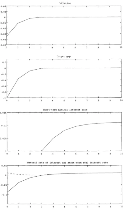
Figure 1 shows the responses of various variables to an adverse shock to the natural rate of interest in the case of discretion.19 In the baseline case, shown in this figure, we assume that the initial shock to the natural rate of interest, ?e in Equation (8), is equal to -0.10, which means a 40% decline in the annualized natural rate of interest. In addition, we assume that the persistence of the shock, which is represented by p in Equation (8), is 0.5 per a quarter. The path of the natural rate of interest is shown at the bottom of Figure 1. In response to this shock, the short-term nominal interest rate is set to zero for the first four periods until period 3, and is positive in period 4 when the natural rate of interest turns positive. Inflation and the output gap take negative values for the first four periods during which a zero interest rate policy is adopted, and return to the steady-state value (i.e., zero) in and after period 4.
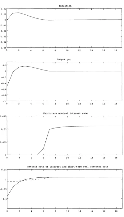
Figure 2 shows the responses of the same set of variables in the case of commit- ment.20 An important difference from the case of discretion is that a zero interest rate policy is continued longer, which is consistent with Equation (35). A prolonged zero interest rate policy lowers the long-term interest rate during the first six periods. This reduces the central bank's losses in periods 0-3, during which the natural rate of interest is negative, by alleviating deflationary pressures, while it increases losses in periods 4 and 5 by creating positive inflation and output gap. It is also important to note that the cumulative sum of the deviation of the short-term real interest rate from the natural rate of interest during the periods of zero interest rate policy is negative, although significantly smaller than in the case of discretion. This implies that a zero interest rate policy would be extended further if we follow the augmented Taylor rule, proposed by Reifschneider and Williams (2000), which requires that the deviation should be zero, on average, during the periods of zero interest rate policy. Table 2 compares Td and Tc for various combinations of p and e0. If a shock to the natural rate of interest is small and non-persistent, the difference between the two is negligibly small (see, for example, the case of en = -0.02 and p = 0). However, given the value of p, the difference between the two becomes larger with the absolute value of eo. In the case of p = 0, for example, Td and Tc coincide when e4 = -0.02, but the difference between the two emerges and increases as eg becomes larger in absolute value. On the other hand, given the size of the shock, a change in its persistence does not affect the difference between the two, although both Td and Tc increases with p.
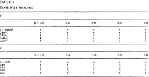
Finally, to check the sensitivity of the results, Table 3 computes Tc changing parameter values for 3, X, K, and a within a plausible range. Note that Td is equal
19. We use MATLAB 5.3.1 for the calculation.
20. A key part in computing the commitment solution is how to find the timing to terminate a zero interest rate policy, Tc. We search Tc as follows: (1) we set Tc at a sufficiently high value, say 50, under which ljTC is supposed to be negative, and compute the path of the variables; (2) if OlTC is negative, we try Tc = 49; and (3) we repeat this until 1ITC becomes non-negative.
0 -
-0.01-
-0.02-
-0.03-
-0.04
-0.05
0 1 2 3 4 5 6 7 8 9 10
Output gap
0.2-
0 -
-0.2- /
-0.4-
-0.6- -0.8-
-1 I I
0 1 2 3 4 5 6 7 8 9 10
Short-term nominal interest rate
0.01-
0.005-
0 1 2 3 4 5 6 7 8 9 10
Natural rate of interest and short-term real interest rate
0
-0.05
-0.1
0 1 2 3 4 5 6 7 8 9 10
FIG. 1. Optimal Responses under Discretion
I I I I I i I I I
015 I I I I I I l I
( I.I..
:1 I I I I I I I I I
I I . I . . .
I I I , I I I
- - - -
0.01
-0.01-
-0.02- -0.03 - -0.04- -0.05 0 5
0 2 4 6 8 10 12 14 16 18
Output gap 0.2-
o- -0.2 -0.4 -0.6- -0.8- -1
0 2 4 6 8 10 12 14 16 18
Short-term nominal interest rate
0.015 I I I I I
0.01-
0.005-
0 2 4 6 8 10 12 14 16 18
Natural rate of interest and short-term real interest rate
0.05 1 , 1 1 , I I I
0-
-0.05
-0.1-
2 4 6 8 10 12 14 16 18
FIG. 2. Optimal Responses under Commitment
-
I I'
TABLE 2
VARIOUS TYPES OF SHOCK
Td
= -0.02 -0.05 -0.10 -0.20 -0.30
p = 0.7 1 4 6 8 9
0.5 0 2 3 4 4
0.3 0 1 1 2 2
0.1 0 0 0 1 1
0.0 0 0 0 0 0
TC
" = -0.02 -0.05 -0.10 -0.20 -0.30
p = 0.7 2 6 9 11 13
0.5 1 3 5 7 8
0.3 0 2 3 5 6
0.1 0 1 2 4 5
0.0 0 1 2 3 4
to 3, independent of these parameter values. As seen in the table, TC indeed changes depending on parameter values, ranging from 3 to 6,21 but exceeds Td, which is equal to 3, in almost all cases. In this sense, the result we saw in the previous section that TC is greater than Td holds, not only qualitatively, but also quantitatively.
TABLE 3
SENSITIVITY ANALYSIS
TC
p = 0.99 0.97 0.95 0.93 0.91
3 = 0.05/42 5 5 5 5 5
0.10/42 5 5 5 5 5
0.15/42 4 4 4 4 4
0.20/42 4 4 4 4 4
0.25/42 3 3 3 3 3
TC
K = 0.02 0.04 0.06 0.08 0.10
o = 0.05 3 4 4 4 4
0.10 5 5 4 4 4
0.15 5 5 5 5 5
0.20 5 5 5 5 5
0.25 6 5 5 5 5
NOTE: e' = -0.10; = 0.5.
21. The upper part of the table shows that TC decreases as X increases, whereas changes in P within a plausible range have no impact on Tc. Moreover, the lower part of the table shows that TC decreases as K increases while TC increases as ( increases. These results are consistent with the qualitative results we saw in the previous section.