NATURE|VOL 419|12 SEPTEMBER 2002|www.nature.com/nature 2 0 7
T
he world ocean is one of the main constituents of the climate system and affects climate in a multitude of ways. Its sheer size is obvious: 71% of the Earth is covered by ocean, so that most of the solar radiation received at the Earth’s surface goes into the ocean and warms the surface waters. As a result of its heat capacity and circulation, the ocean has the ability to both store and redistribute this heat before it is released to the atmosphere (much of it in form of latent heat, that is, water vapour) or radiated back into space.The heat storage effect is most apparent on the seasonal timescale. The mid-latitude temperature range between summer and winter is typically around 8 7C over the ocean and at the coast, whereas this range is up to several tens of degrees in the continental interiors (see Figure 2.1 in ref. 1, which contours the observed seasonal tempera- ture range).
A corresponding figure for the temperature deviation from the zonal mean (Fig. 1 in ref. 2) gives an indication of
the effect of ocean heat transport on surface temperatures, with warm anomalies over the three main regions of deep- water formation of the world ocean: the northern North Atlantic, the Ross Sea and the Weddell Sea. These are key areas for the thermohaline circulation of the world ocean (see Box 1), where surface waters after releasing heat to the atmosphere reach a critical density and sink. Clearly not all deviations from zonal mean conditions are due to ocean circulation, but the magnitude of the warm anomaly over the northern North Atlantic (~ 10 7C) is in agreement with estimates3and simulations of climate models4–7of the effect of ocean heat transport (Fig. 1).
In addition to its heat storage and transport effects, the ocean can influence the Earth’s heat budget by its sea-ice cover, which changes the planetary albedo and can thus affect the steady-state global-mean temperature. Sea ice also acts as an effective thermal blanket, insulating the ocean from the overlying atmosphere. This is so effective that in a typical ice-covered sea more than half of the air–sea heat
Ocean circulation and climate
during the past 120,000 years
Stefan Rahmstorf
Potsdam Institute for Climate Impact Research, PO Box 601203, 14412 Potsdam, Germany
Oceans cover more than two- thirds of our blue planet. The waters move in a global circulation system, driven by subtle density differences and transporting huge amounts of heat. Ocean circulation is thus an active and highly nonlinear player in the global climate game. Increasingly clear evidence implicates ocean circulation in abrupt and dramatic climate shifts, such as sudden temperature changes in Greenland on the order of 5–10 7C and massive surges of icebergs into the North Atlantic Ocean — events that have occurred repeatedly during the last glacial cycle.
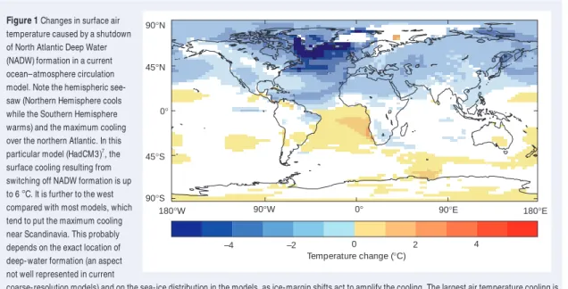
Figure 1Changes in surface air temperature caused by a shutdown of North Atlantic Deep Water (NADW) formation in a current ocean–atmosphere circulation model. Note the hemispheric see- saw (Northern Hemisphere cools while the Southern Hemisphere warms) and the maximum cooling over the northern Atlantic. In this particular model (HadCM3)7, the surface cooling resulting from switching off NADW formation is up to 6 7C. It is further to the west compared with most models, which tend to put the maximum cooling near Scandinavia. This probably depends on the exact location of deep-water formation (an aspect not well represented in current
coarse-resolution models) and on the sea-ice distribution in the models, as ice-margin shifts act to amplify the cooling. The largest air temperature cooling is thus greater than the largest sea surface temperature (SST) cooling. The latter is typically around 5 7C and roughly corresponds to the observed SST difference between the northern Atlantic and Pacific at a given latitude. In most models, maximum air temperature cooling ranges from 6 7C to 11 7C in annual mean; the effect is generally stronger in winter.
–4 –2 0 2 4
180°W 90°W 0° 90°E 180°E
90°N
90°S 45°S 45°N
0°
Temperature change (°C)
exchange occurs through patches of open water (leads) that make up around 10% of the surface area.
Finally, the ocean affects the climate system not only by being part of the planetary energy cycle, but also by participating in the biogeo- chemical cycles and exchanging gases with the atmosphere, thus influencing its greenhouse gas content. For example, the ocean contains about fifty times more carbon than the atmosphere, and theories seeking to explain the lower concentrations of atmospheric carbon dioxide that prevailed during glacial times invariably invoke changes in the oceanic carbon sink, either through physical or biolog- ical mechanisms (the so-called ‘biological pump’).
Rather than providing a general overview of the ocean’s role in the climate system, which is a subject matter for textbooks, I focus here on the role of ocean circulation changes in major climate changes during the past 120,000 years, since the Eemian interglacial. This is a period for which palaeoclimatic data of relatively good global coverage and dating are available. The emphasis is on presenting physical ideas and con- cepts for understanding these climate changes; more-detailed reviews of the palaeoclimatic data can be found elsewhere (see, for example, refs 8–10). This is a highly dynamical research field with rapid progress, but not yet a generally accepted and established theory. Controversies remain over many issues, and the interpretation I have attempted here is subjective and will probably turn out to be partly wrong.
Reconstructing past ocean circulation
Analysis of sediment cores and corals provides a wealth of informa- tion on past ocean circulation, and clearly shows that it has
undergone significant changes during the past 120,000 years. Reconstructions of past ocean temperatures can be derived, for example, from species abundances of fossil plankton, from organic geochemistry (using alkenone unsaturation indices), from trace- metal ratios (Sr/Ca, U/Ca or Mg/Ca) in corals or calcite shells, and to some extent from oxygen isotopes. Using multiple proxies, informa- tion on salinity can also be reconstructed. This constrains the distribution and properties of water masses; information on flow rates is harder to obtain. Indirect evidence for ventilation rates comes from the distribution of isotopes such as 13C (ref. 11) or radiochemi- cal tracers12, and from the radiocarbon content of the atmosphere. In some locations, the grain size of sediments yields information on the speed of local bottom currents13, or density gradients have been reconstructed to give information on the geostrophic current component14. Although there is still much discussion on the interpretation and error margins of each data type, and in some cases proxy data seem to give contradictory results, an increasingly consistent picture is emerging.
Time-slice compilations suggest that at different times, three dis- tinct circulation modes have prevailed in the Atlantic15,16(Fig. 2). These have been labelled the stadial mode, interstadial mode and Heinrich mode (based on their occurrence during stadial and inter- stadial phases of glacial climate and during Heinrich events), or the cold, warm and off mode (based on their physical characteristics in the North Atlantic). In the interstadial mode, North Atlantic Deep Water (NADW) formed in the Nordic Seas, in the stadial mode it formed in the subpolar open North Atlantic (that is, south of Iceland), whereas Box 1
Some key facts about ocean circulation
The large-scale ocean circulation can be thought of as a combination of currents driven directly by winds (mostly confined to the upper several hundred metres of the sea), currents driven by fluxes of heat and freshwater across the sea surface and subsequent interior mixing of heat and salt (the so-called thermohaline circulation), and tides (driven by the gravitational pull of the Moon and Sun). These driving mechanisms interact in nonlinear ways (since all currents change the heat and salt distribution) so that no unique decomposition exists. Nevertheless the distinction is useful, particularly when changes in wind or in surface heat and freshwater fluxes are considered for their effects on the circulation.
An important way in which wind-driven currents are thought to lead to climatic changes is through their effect on upwelling (Ekman divergence) near coasts and the Equator, changing sea surface temperatures. This mechanism plays a part in the El Niño/Southern Oscillation cycle. The thermohaline circulation is most interesting for its highly nonlinear response to changes in surface freshwater forcing88, allowing large changes in heat transport to occur (see Box 2). Tides are relevant to the climate system because they form one of the main sources of turbulent energy (in addition to that provided by the wind) to mix the ocean89.
A highly simplified cartoon of the global thermohaline circulation (sometimes called ‘conveyor belt’) is shown in the figure above (modified from the original by Broecker). Near-surface waters (red lines) flow towards three main deep-water formation regions (yellow ovals) — in the northern North Atlantic, the Ross Sea and the Weddell Sea — and recirculate at depth (deep currents shown in blue, bottom currents in purple; green shading indicates salinity above 36‰ , blue shading indicates salinity below 34‰ ). A recent estimate of the rate of deep-water formation is 1552 Sv (1 Sv4106m3s–1) in the North Atlantic and 2156 Sv in the Southern Ocean90. Northward heat transport into the northern Atlantic peaks at 1.350.1 PW (1 PW41015W) in the subtropics90; this heat transport warms the northern Atlantic regional air temperatures by up to 10 7C
over the ocean with the effect declining inland.
Little is currently known about present-day natural variability of this circulation (see ref. 91 for a review), or about the effects of such variability on surface climate. Variations of the Atlantic thermohaline circulation on timescales of several decades are found in many coupled climate models, with a typical amplitude of a few sverdrup; they are probably damped oscillations driven by stochastic variations in surface fluxes (that is, weather variability)92. Good observational time series of integral measures of this circulation are lacking, although some data suggest that such decadal variability also exists in nature, and is correlated with the North Atlantic Oscillation (NAO)93,94. The NAO also seems to orchestrate the location and intensity of deep convection in the northern Atlantic95. Lack of data makes it hard to establish whether a longer-term trend in the circulation exists, although there is intriguing evidence for trends in temperature and salinity96,97that may indicate a gradual weakening of the overflow from the Nordic Seas into the Atlantic in recent decades.
NATURE|VOL 419|12 SEPTEMBER 2002|www.nature.com/nature 2 0 9 in the Heinrich mode NADW formation all but ceased and waters of
Antarctic origin filled the deep Atlantic basin. This grouping of the data in three distinct modes is a somewhat subjective interpretation. However, it is clear that latitude shifts of convection (between the Nordic Seas and the region south of Iceland) have occurred16,17, and that at certain times (for example, during Heinrich events) NADW formation was interrupted11,18. There is also firm evidence now for a link between these changes in ocean circulation and changes in surface climate (argued in more detail in refs 8, 19).
Modelling past climate and ocean changes
Numerical models of the climate system are essential in the forma- tion and exploration of quantitative hypotheses about the dynamics of climate changes; the system is too complex to be understood by heuristic arguments or analytical calculations. Numerical models incorporate and combine our knowledge about many individual physical processes in a quantitative way. Obviously, knowledge about these processes is incomplete and often inaccurate, and each model is a compromise as to how many processes are included, at what level of complexity and with what resolution20, given limited computer and human resources. A critical appraisal of what can be learnt from a particular (necessarily imperfect) model experiment thus involves not only looking at the result, but also understanding exactly how it was obtained. For this reason, non-specialists sometimes suspect that models are either notoriously wrong or ‘can be tuned to do anything’. (In fact, ‘tuning’ to determine the optimal values for certain model
parameters is an essential part of constructing a good model; a set of rules for good tuning practice is proposed in ref. 21.)
Nevertheless, models have now reached a level where useful and fairly realistic simulations of many aspects of palaeoclimate have become possible, so that a quantitative understanding of key mechanisms and feedbacks in past climate changes is emerging. On the other hand, palaeoclimatic reconstructions of past climatic forcings and the resulting changes in atmospheric and oceanic conditions are now advanced enough to provide a challenging test bed for the performance of climate models. This is an important credibility test for models that are also used for estimating the effects of anthropogenic climate forcing from increasing concentrations of greenhouse gases.
A landmark was reached with the first simulations of a radically different climate, that of the Last Glacial Maximum (LGM), with cou- pled ocean–atmosphere models from prescribed orbital, CO2and continental ice-sheet forcing22–25. The huge computing requirements of this task, resulting from the long timescale of adjustment of the ocean circulation (several thousand years), were overcome in differ- ent ways: by using fast models of intermediate complexity22,23, by studying only the initial adjustment to the forcing24, or by brute force, running the model for over a year on a supercomputer25. These models confirm the result of the much cheaper, atmosphere-only sim- ulations of glacial climate (see, for example, ref. 26) that, given these forcings, the high albedo of the continental ice sheets and the low CO2 concentrations are the dominant factors leading to a global cooling. In addition, the coupled models predict the state of the ocean circulation and the effect of oceanic changes on surface climate. For example, two of the models22,25obtained a southward shift of NADW formation in glacial climate, as is suggested by sediment data16,17.
Glacial inception
The first of the major climatic changes considered here is the transi- tion from the Eemian interglacial to the beginning of glacial climate, which occurred between 120,000 years (120 kyr) and 115 kyr ago. Data for the Eemian climate are too scarce to build a reliable picture, but global simulations of Eemian climate together with local palaeodata suggest it may have been around 1 7C warmer (global annual mean) compared with the modern pre-industrial climate27, with particularly warm temperatures in Northern Hemisphere summers. Sea-level reconstructions28 show that climate moved rapidly from this state into the last glacial, reaching almost half of the glacial-maximum ice volume within a few thousand years (see review in this issue by Lambeck et al., pages 199–206). The challenge of understanding this shift has become known as the ‘glacial inception problem’.
The cause for this climate shift must be the Milankovich cycles of the Earth’s orbit around the Sun, which are believed to be the ultimate forcing for the glacial cycles of the past 2 million years. At 115 kyr ago, summer insolation at high northern latitudes was up to 40 W m–2less than at present. Simple, nonlinear conceptual models29are able to
‘Cold’
‘Off’
Depth (km)Depth (km)Depth (km)
‘Warm’ 0
1 2 3 4 5 0 1 2 3 4 5 0 1 2 3 4
530°S 0 30°N 60°N 90°N
Figure 2Schematic of the three modes of ocean circulation that prevailed during different times of the last glacial period. Shown is a section along the Atlantic; the rise in bottom topography symbolizes the shallow sill between Greenland and Scotland. North Atlantic overturning is shown by the red line, Antarctic bottom water by the blue line.
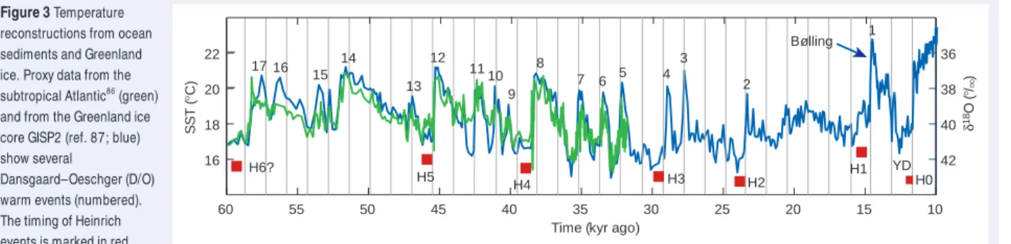
Figure 3Temperature reconstructions from ocean sediments and Greenland ice. Proxy data from the subtropical Atlantic86(green) and from the Greenland ice core GISP2 (ref. 87; blue) show several
Dansgaard–Oeschger (D/O) warm events (numbered). The timing of Heinrich events is marked in red.
Grey lines at intervals of 1,470 years illustrate the tendency of D/O events to occur with this spacing, or multiples thereof.
60 55 50 45 40 35 30 25 20 15 10
42 40 38 36
16 18 20 22
1
2 3 5 4 7 6 8 9 1110 12 13 14 16 15 17
H1 YD
H5 H4 H3 H2 H0
Time (kyr ago)
SST (°C) δ18O (°/°°)
Bølling
H6?
sheets: a strong circulation warms the northern Atlantic and melts surrounding ice, which leads to meltwater runoff and weakens the circulation again36,40. These were conceptual ideas, but circulation models are also able to show several types of internal oscillations in thermohaline flow (without ice sheets) under certain forcing condi- tions41. The relevance of such model oscillations for the real ocean is open to debate, and a problem of all internal-oscillation theories for D/O events is to explain the waiting-time statistics found by Alley and co-workers.
A third idea is that of latitude shifts of convection3between Nordic Seas and the mid-latitude open Atlantic Ocean. Based originally on sediment data, this idea has found strong support in model simula- tions showing that such a mechanism can explain many observed features of D/O events42, including the three-phase time evolution, reproduce the observed glaciations from this forcing (according to
these, the next glaciation can be expected in ~ 30 kyr from now). A number of climate models have been used to study glacial inception even without incorporating a continental ice-sheet model, based on the concept that snow cover that persists through- out the summer would eventually grow into an ice sheet. Discussion has focused on the conditions under which sufficient perennial snow cover can be achieved. This has turned out to be difficult in atmosphere-only models with present-day sea surface temperatures and vegetation cover. A reduction in high-latitude forest cover greatly increases the albedo after snowfall, leading to a positive snow-albedo feedback that helps glacial inception30. Lower high- latitude sea surface temperatures (caused by the insolation change) are also clearly conducive to perennial snow cover31. Recently, a real- istic simulation of glacial inception in terms of actual ice-sheet growth has been achieved in an Earth system model of intermediate complexity that includes a continental ice-sheet model (R. Calov & A. Ganopolski, in preparation).
Does a weakening in Atlantic Ocean circulation have a role in glacial inception? There are no palaeoclimatic data showing that NADW formation slowed at this time. Model simulations that include a dynamical ocean model achieve glacial inception with only minor changes in ocean circulation (ref. 31; and R. Calov & A. Ganopolski, in preparation) — changes that are too small to be important in glacial inception in these models. The reverse theory32, namely that a warm North Atlantic could have induced ice-sheet growth by enhanced moisture supply, goes against our knowledge of glacier mass balance: glaciers grow when climate is cold, not warm and moist.
Dansgaard–Oeschger events
Dansgaard–Oeschger (D/O) events (Figs 3, 4) are perhaps the most pronounced climate changes that have occurred during the past 120 kyr. They are not only large in amplitude, but also abrupt (irre- spective of whether one follows a physical definition of abruptness33 or takes it to mean ‘in less than 30 years’8). In the Greenland ice cores, D/O events start with a rapid warming by 5–10 7C within at most a few decades, followed by a plateau phase with slow cooling lasting several centuries, then a more rapid drop back to cold stadial condi- tions. The events are not local to Greenland (Fig. 3); a comprehensive review of spatial coverage (for events during marine isotope stage 3, 59–29 kyr ago) is given by Voelker et al.10who list 183 sites, most of which clearly show these events (Fig. 4). Amplitudes are largest in the North Atlantic region, and many Southern Hemisphere sites, especially those in the South Atlantic, reveal a hemispheric ‘see-saw’ effect (cooling while the north is warming). Alley et al.34have shown that these events have curious statistical properties: the waiting time between two consecutive events is often around 1,500 years, with further preferences around 3,000 and 4,500 years (Fig. 3), which suggests a stochastic resonance35process at work.
Several ideas have been advanced to explain D/O events, most of which involve the thermohaline circulation of the Atlantic. The first of these was probably the idea of thermohaline circulation bistability36: NADW formation is active during the warm phases (interstadials), whereas it is shut off during cold phases (stadials), and some outside trigger causes mode switches between these two stable states. This idea is based on the bistability of the circulation for modern climate in models (Broecker36cites the bistability found in Stommel’s37classic model; see Box 2). However, this theory is at odds with more recent sediment data showing NADW formation active during stadials12,15 and shut down only during or after Heinrich events11,18.
A second idea is that of internal oscillations in the volume trans- port of the thermohaline circulation. Broecker’s salt oscillator38is based on the (challenged39) notion that the Atlantic thermohaline circulation balances the net atmospheric freshwater export from the Atlantic basin. A weakening of the circulation would thus lead to a salinity build-up in the Atlantic, strengthening the circulation again. A variation of this idea involves the surrounding continental ice
The thermohaline circulation is thermally driven: highest surface densities in the world ocean are reached where water is coldest, in spite of the lower salt content there compared with the warmer tropical and subtropical regions. Nevertheless, the influence of salinity is important and is the main cause of the nonlinearity of the system. Salinity is involved in a positive feedback. Higher salinity in the deep-water formation area enhances the circulation, and the circulation in turn transports higher salinity waters into the deep- water formation regions (which tend to be regions of net precipitation, that is, freshwater would accumulate and surface salinity would drop if the circulation stopped). This leads to two possible equilibrium states, with and without North Atlantic Deep Water (NADW) formation4. This was first described in a classic paper by Stommel37with the help of a simple box model.
The stability properties are illustrated in the diagram below, which plots the strength of the thermohaline circulation as a function of the freshwater input into the North Atlantic. The simple
presentation shows the bistable regime and a saddle-node bifurcation point where the circulation breaks down (for a more detailed discussion, see ref. 88).
This salt-transport feedback is not the only feedback rendering the system nonlinear. The convective mixing process at high latitudes is itself a highly nonlinear, self-sustaining process, which at least in models can lead to multiple stable convection patterns3,98. Together, these two positive feedback mechanisms allow two types of transitions between distinct circulation modes: on/off switches of NADW formation, and shifts in the location of convection. These two mechanisms are crucial in attempts to explain glacial climate changes.
The thermohaline circulation takes several thousand years to reach full equilibrium. The transient response to a change in forcing can therefore deviate substantially from the equilibrium solutions and is in many cases more linear99.
Box 2
Stability and nonlinearity of the thermohaline circulation
Freshwater forcing (Sv)
–0.1 0 0.1
NADW flow (Sv) 20 0
Stommel bifurcation Present
climate?
Bistable regime
NATURE|VOL 419|12 SEPTEMBER 2002|www.nature.com/nature 2 1 1 spatial pattern and hemispheric see-saw. In this mechanism, the rapid
warming phase results from a northward intrusion of warm Atlantic waters into the Nordic Seas, the plateau phase is the ‘warm mode’ of Atlantic Ocean circulation (see above), which gradually weakens over several centuries, and the final cooling phase marks the end of deep- water formation in the Nordic Seas. Some trigger is required to start the event, the exact nature of which remains unknown. However, because this is a threshold mechanism it lends itself naturally to stochastic resonance, with random climate variability plus a weak external cycle in freshwater forcing (for example, driven by a solar cycle43,44) combining to cross the critical threshold45,46.
Finally, the tropical driver hypothesis47,48does not involve changes in thermohaline circulation, but suggests that D/O-style tempera- ture shifts in Greenland may be caused by shifts in the atmospheric planetary-wave pattern, controlled remotely from the tropics. This is based on the strong control that tropical sea surface temperatures exert over global atmospheric heat-transport patterns in present climate, but a more specific and quantitative explanation for D/O events building on this idea is yet to emerge.
It is possible that several of these basic physical ideas work togeth- er in D/O events. For example, shifts in convection latitude could be caused by changes in atmospheric freshwater transport controlled partly from the tropics.
Heinrich events
Heinrich events are the second major type of climatic event that occurred mostly in the latter half of the last glacial. They are
characterized by distinct layers in North Atlantic sediments49,50, spaced at irregular intervals of the order of 10,000 years. Sediments in these layers are so coarse that they can only have been transported out into the ocean by icebergs; hence, they are referred to as ice-rafted debris. The thickness of these layers, decreasing from several metres in the Labrador Sea down to a few centimetres in the eastern Atlantic, strongly suggests that Heinrich events are massive episodic iceberg discharges from the Laurentide ice sheet through Hudson Strait, with up to 10% of the ice sheet sliding into the ocean51–53. A highly plausible explanation is that the ice sheet grew to a critical height where it became unstable, and a major surge could then start spontaneously or be triggered by a small perturbation54,55. Sediment data show that NADW formation ceased or was at least strongly reduced during Heinrich events11,15,56, and models consistently show that this is to be expected6,42,57–60given the reduction in surface water density associated with such a large freshwater release (up to 0.1 Sv; ref. 53).
The climatic consequences of Heinrich events thus probably consist of the superposition of two effects: the direct effect of the ice- sheet surge, leading to a lowered ice sheet and higher sea level, and the effect of the subsequent breakdown of the Atlantic thermohaline circulation. The climate signature of Heinrich events differs from D/O events in several ways. In Greenland, stadials were equally cold with or without Heinrich events. Further south around the Atlantic, however, Heinrich events manifest as clear cold intervals with even larger amplitude than D/O warmings61–63. This pattern can be explained if the ‘latitude shift of convection’ theory of D/O events is
180˚ W 120˚ 60˚ 0˚ 60˚ 120˚ 180˚ E
60˚ S 30˚ 0˚ 30˚ 60˚ N
180˚ W 120˚ 60˚ 0˚ 60˚ 120˚ 180˚ E
60˚ S 30˚ 0˚ 30˚ 60˚ N Wind
SSTNPIW OMZ
Humid
SST IRD input SST SSS
SSTDW
SST
% NADW Prod.
SW mons.
Humid
Humid Wind DW
Prod. Humid
Ventilated LCDW
Summer mons.
Cooling Cooling
Warming
Warming Arid
SST Humid
Wind
SST DW
Prod. Prod.
% NADW
NE mons. Winter mons. SST
NPIW OMZ
Grasland expansion Arid Sporadic IRD
IRD SSTSSS SST
SST TCO CH24
DW
TCO CH42
TCO CH24 SST
SST
SST Prod. SST T
T
T T T
Humid Humid
T T
SST
Upwelling Drier cond.
Wind
T
TCO CH24 Dust IRD
SSTSSS
SST AridT
% AABW SST SST % AABW
SST SST Arid Prod.
T T
Arid Arid
SSSSST GNAIW T
Humid
Forest expansion T
T
SST SST
% NADW
% NADW Upwelling
SST a
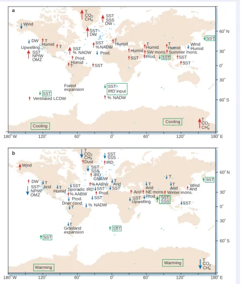
b Figure 4Overview of palaeoclimatic proxy data10
characterizing warm phases (top) and cold phases (bottom) during marine oxygen isotope stage 3 (MIS-3; 59–29 kyr ago, compare with Fig. 3). Red arrows (blue arrows) indicate trends, that is, warmer (colder), more (less) or increased (lowered). Green text and arrows indicate trends opposite to the general climate conditions. Abbreviations: T, temperature; SST, sea surface temperature; SSS, sea surface salinity; mons., monsoon; prod., productivity; cond., conditions; IRD, ice-rafted debris; OMZ, oxygen minimum zone. Water masses are labelled as follows: DW, Deep Water; NADW, North Atlantic Deep Water; AABW, Antarctic Bottom Water; NPIW, North Pacific Intermediate Water; LCDW, Lower Circumpolar Deep Water; GNAIW, Glacial North Atlantic Intermediate Water.
Greenland ice core GISP2, this follows almost exactly 9 kyr after D/O 2, thus fitting a multiple of the 1,500-year cycle.
Synchronous with the Bølling warming is a small cooling in Antarctica — the Antarctic cold reversal — which interrupts the general trend towards warming there, and which represents the characteristic see-saw response to the change in Atlantic Ocean circu- lation associated with D/O 1. A major inflow of meltwater74into the ocean (meltwater pulse 1A) is registered shortly after the strong northern warming. This could be a consequence of the Bølling warming, assuming most of this meltwater originated from the northern ice sheets (a question that is debated). But the meltwater did not immediately close down NADW formation, perhaps because it did indeed originate mostly in the Southern Hemisphere, or perhaps because the North Atlantic was at this time in the vigorous warm interstadial mode, which is relatively insensitive to freshwater forcing. D/O 1 finally ended (as did the previous D/O events), giving way to the Younger Dryas (YD) cold event (warming accelerates in Antarctica at this point). Finally, at 11.5 kyr ago, the YD ends with an abrupt warming that might be called D/O 0, almost exactly 3 kyr after D/O 1, again fitting the 1,500-year pattern. This warming is also followed by another major meltwater pulse (pulse 1B), but this time the North Atlantic remains in the warm circulation mode, which is stable in warmer climates and prevails in the Holocene.
Model simulations with the CLIMBER-2 model show that this is a feasible scenario that can be reproduced from prescribed insolation, CO2, ice-sheet and meltwater forcing. However, the sequence and timing of events is particularly sensitive to the details of the freshwa- ter forcing, which are poorly known. Efforts have been made to estimate the history of meltwater flux from different outlets and link it to ocean circulation and climate changes73, but additional data are needed to obtain a more robust representation, and the freshwater forcing may never be known accurately enough to allow truly deterministic modelling.
The Younger Dryas event seems to be special in a number of ways. Because of the high meltwater influx at this time, NADW formation probably stopped58,75,76, as during Heinrich events. Nevertheless, it seems hard to reconcile the fact that the Younger Dryas event is almost as cold as previous Heinrich events during glacial-maximum conditions with the already elevated CO2level in the atmosphere (over 240 p.p.m.) and reduced inland ice volume. Furthermore, there is increasing evidence from New Zealand77and South America78,79 that the Younger Dryas event was accompanied by a global re- advance of ice, which is also reflected in a temporary halt of sea-level rise28. The Younger Dryas event may thus be more than a change in ocean circulation; a global forcing causing cooling could be involved, possibly of solar origin80.
A final northern cooling in the history of deglaciation is a short event occurring 8,200 years ago, which has also been linked to a meltwater-induced weakening of the thermohaline circulation81. El Niño/ Southern Oscillation
In present-day climate, the strongest mode of natural climate variability is the El Niño/Southern Oscillation (ENSO). It is a cou- pled ocean–atmosphere mode centred on the tropical Pacific, with a variable period of 3–7 years and worldwide ecological and societal impacts due to its effect on the global atmospheric circulation. Annually banded corals provide a unique opportunity to determine whether this mode has also been in operation during different climatic states of the past, as they record climatic information at up to monthly resolution in the chemistry of their skeletons as they grow82. As a result of tectonic uplift, fossil coral reefs from past climatic peri- ods can be found on exposed terraces at some sites, such as the Huon Peninsula of Papua New Guinea (see review in this issue by Lambeck et al., pages 199–206).
Coral data from different time segments show convincingly that ENSO variability prevailed in very different climates, including glacial times and the Eemian interglacial82. The amplitude seems to correct: during stadials, the ocean is in the ‘cold mode’ with the warm
Atlantic current stopping too far south to warm Greenland, so that shutting it down has no effect there42(but it does further south).
The data further show that at most Antarctic sites, Heinrich events are associated with warming that is stronger than that during other stadials64. This is the bipolar see-saw (or ‘sea-saw’) effect65,66, resulting from the reduced interhemispheric heat transport by the ocean; the effect of a shutdown of NADW formation is greater than that of a latitude shift42. There are in fact two see-saw effects in opera- tion: in addition to the temperature see-saw, many models indicate there is a deep-water formation see-saw, which will lead to enhanced Southern Ocean deep-water formation if NADW formation is reduced, and vice versa. As well as enhancing the see-saw response in temperature, this mechanism gives a possible role to changes in the Southern Ocean deep-water source in affecting northern Atlantic climate67.
D/O and Heinrich events are not unrelated. First, each Heinrich event is followed by a particularly warm D/O event; successive D/O events tend to get progressively cooler until the next Heinrich event (this sequence of D/O events is sometimes referred to as a Bond cycle). This could simply be a consequence of the Laurentide ice sheet growing gradually in height between Heinrich events.
Second, Heinrich events apparently always occur during cold sta- dials and not in the warm phase of D/O events51. This suggests that ice-sheet instability does not occur at random, but is helped by some climatic trigger, possibly a temperature or sea-level change68; there is also evidence for smaller precursor events69. The issue of a possible trigger mechanism, which may also synchronize discharges from separate ice sheets68, is one of the important, currently open research questions surrounding Heinrich events.
Deglaciation and the Younger Dryas event
The end of the last ice age and the transition to the Holocene is the last first-order global climatic change on record. Since then, climate has been relatively warm and stable, providing a conducive environment for the development of human civilization. A rise in (ice-volume- equivalent) sea level by 130 m between 19 kyr and 7 kyr ago marks the rapid vanishing of the glacial ice sheets28. Many puzzles surround the complex sequence of events that occurred during deglaciation, and three key factors need to be considered: the changes in insolation (due to the Milankovich cycles) which must have initiated deglacia- tion, the rise in atmospheric CO2levels providing a strong global warming feedback, and changes in ocean circulation.
Surface warming started around 17–20 kyr ago in Antarctica and proceeded approximately synchronously with the rise in atmospher- ic CO2and global sea level. Northern records such as the Greenland ice cores, however, show a very different deglaciation history. A consistent and plausible (although tentative) explanation can be advanced if we assume (as for the D/O and Heinrich events discussed above) that these northern sites are dominated by the state of the Atlantic thermohaline circulation, which went through some signifi- cant changes during deglaciation, in part because of the influx of meltwater from the shrinking ice sheets.
According to this explanation, warming from glacial-maximum conditions is initiated by changes in northern insolation70(summer insolation increases in high latitudes of the Northern Hemisphere by about 30 W m–2between 24 and 12 kyr ago). The carbon cycle responds almost synchronously by releasing CO2to the atmos- phere71, which reinforces and globalizes the warming (together with other greenhouse gases, primarily water vapour), and the ice sheets start to melt. Greenland, however, remains cold (although some warming begins at a similar time as in Antarctica when the two regions are viewed on a common timescale72), as meltwater influx and Heinrich event 1 tend to keep the Atlantic Ocean in cold circula- tion mode73. Greenland then warms abruptly at 14.6 kyr ago in the Bølling warming, owing to a northward shift in ocean circulation (that is, D/O event 1). If we believe the chronology derived from the
NATURE|VOL 419|12 SEPTEMBER 2002|www.nature.com/nature 2 1 3 have varied, however, with particularly weak ENSO variations dur-
ing the mid-Holocene (6.5 kyr ago) and the early glacial (112 kyr ago) and the strongest ENSO during modern times. First attempts to simulate the effect of Milankovich cycles on ENSO variations using a simple model suggest that the precession cycle could directly alter ENSO intensity by zonally asymmetric heating of the equatorial Pacific83. But comparison with data shows that this cannot be the only effect82, and both more data and further simulations with more com- prehensive models are needed to understand ENSO variations through time.
Outlook
The study of climate variations over the past 120,000 years has reached a state where palaeoclimatic data provide increasingly reliable information on the driving forces and the responses of the climate system, and where distinct climatic events such as glaciation, deglaciation, D/O events or Heinrich events can be characterized in terms of their spatial patterns and evolution over time. Understand- ing the mechanisms behind these climatic changes has moved beyond speculation to specific, testable hypotheses backed up by quantitative simulations.
It has become clear that the climate system is sensitive to forcing and responds with large and often abrupt changes in surface condi- tions. The role of the ocean circulation is that of a highly nonlinear amplifier of climatic changes. Many issues are still controversial and unresolved, both in terms of the data (for example, whether the late-glacial glacier advance in New Zealand and South America is synchronous with the Younger Dryas cold event in the north) and in terms of the mechanisms (for example, whether Younger Dryas cooling is caused by a meltwater-induced shutdown of NADW for- mation). But progress has been rapid, and the potential exists to resolve many of these issues in the coming decade or so by collecting more data, refining the analysis methods and improving models.
A better understanding of the carbon cycle remains one of the main challenges; the ocean has a crucial role in this cycle, one that could not be discussed here owing to space limitations. Reconstruc- tions71,84and modelling85of carbon cycle changes can provide useful constraints on ocean circulation changes, and understanding the glacial–interglacial changes in atmospheric CO2 concentration remains an elusive central piece in the climate puzzle. ■■
doi:10.1038/nature01090
1. Gill, A. E. Atmosphere-Ocean Dynamics (Academic, San Diego, 1982).
2. Rahmstorf, S. & Ganopolski, A. Long-term global warming scenarios computed with an efficient coupled climate model. Clim. Change 43, 353–367 (1999).
3. Rahmstorf, S. Rapid climate transitions in a coupled ocean–atmosphere model. Nature 372, 82–85 (1994).
4. Manabe, S. & Stouffer, R. J. Two stable equilibria of a coupled ocean-atmosphere model. J. Clim. 1, 841–866 (1988).
5. Ganopolski, A. et al. CLIMBER-2: a climate system model of intermediate complexity. Part II: Model sensitivity. Clim. Dynam. 17, 735–751 (2001).
6. Rahmstorf, S. Bifurcations of the Atlantic thermohaline circulation in response to changes in the hydrological cycle. Nature 378, 145–149 (1995).
7. Vellinga, M. & Wood, R. A. Global climatic impacts of a collapse of the Atlantic thermohaline circulation. Clim. Change 54, 251–267 (2002).
8. Clark, P. U., Pisias, N. G., Stocker, T. F. & Weaver, A. J. The role of the thermohaline circulation in abrupt climate change. Nature 415, 863–869 (2002).
9. Mix, A. C., Bard, E. & Schneider, R. Environmental processes of the ice age: land, oceans, glaciers (EPILOG). Quat. Sci. Rev. 20, 627–657 (2001).
10. Voelker, A. H. L. et al. Global distribution of centennial-scale records for marine isotope stage (MIS) 3: a database. Quat. Sci. Rev. 21, 1185–1214 (2002).
11. Elliot, M., Labeyrie, L. & Duplessy, J.-C. Changes in North Atlantic deep-water formation associated with the Dansgaard-Oeschger temperature oscillations (60-10 ka). Quat. Sci. Rev. 21, 1153–1165 (2002).
12. Yu, E.-F., Francois, R. & Bacon, M. P. Similar rates of modern and last-glacial ocean thermohaline circulation inferred from radiochemical data. Nature 379, 689–694 (1996).
13. Bianchi, G. G. & McCave, I. N. Holocene periodicity in North Atlantic climate and deep-ocean flow south of Iceland. Nature 397, 515–517 (1999).
14. Lynch-Stieglitz, J., Curry, W. B. & Slowey, N. Weaker Gulf Stream in the Florida Straits during the Last Glacial Maximum. Nature 402, 644–648 (1999).
15. Sarnthein, M. et al. Changes in east Atlantic deepwater circulation over the last 30,000 years: eight time slice reconstructions. Paleoceanography 9, 209–267 (1994).
16. Alley, R. B. & Clark, P. U. The deglaciation of the Northern Hemisphere: a global perspective. Annu. Rev. Earth Planet. Sci. 27, 149–182 (1999).
17. Oppo, D. & Lehman, S. J. Mid-depth circulation of the subpolar North Atlantic during the Last Glacial Maximum. Science 259, 1148–1152 (1993).
18. Keigwin, L. D. & Lehman, S. J. Deep circulation change linked to Heinrich event 1 and Younger Dryas in a mid-depth North Atlantic core. Paleoceanography 9, 185–194 (1994).
19. Bond, G. et al. Correlations between climate records from North Atlantic sediments and Greenland ice. Nature 365, 143–147 (1993).
20. Claussen, M. et al. Earth system models of intermediate complexity: closing the gap in the spectrum of climate system models. Clim. Dynam. 18, 579–586 (2002).
21. Petoukhov, V. et al. CLIMBER-2: a climate system model of intermediate complexity. Part I: Model description and performance for present climate. Clim. Dynam. 16, 1–17 (2000).
22. Ganopolski, A., Rahmstorf, S., Petoukhov, V. & Claussen, M. Simulation of modern and glacial climates with a coupled global model of intermediate complexity. Nature 391, 351–356 (1998). 23. Weaver, A. J., Eby, M., Fanning, A. F. & Wiebe, E. C. Simulated influence of carbon dioxide, orbital
forcing and ice sheets on the climate of the Last Glacial Maximum. Nature 394, 847–853 (1998). 24. Bush, A. B. G. & Philander, S. G. H. The role of ocean-atmosphere interactions in tropical cooling
during the Last Glacial Maximum. Science 279, 1341–1344 (1998).
25. Hewitt, C. D., Broccoli, A. J., Mitchell, J. F. B. & Stouffer, R. J. A coupled model study of the last glacial maximum: was part of the North Atlantic relatively warm? Geophys. Res. Lett. 28, 1571–1574 (2001). 26. Webb, R. S., Rind, D. H., Lehman, S. J., Healy, R. J. & Sigman, D. Influence of ocean heat transport on
the climate of the Last Glacial Maximum. Nature 385, 695–699 (1997).
27. Kubatzki, C., Montoya, M., Rahmstorf, S., Ganopolski, A. & Claussen, M. Comparison of the last interglacial climate simulated by a coupled global model of intermediate complexity and an AOGCM. Clim. Dynam. 16, 799–814 (2000).
28. Lambeck, K. & Chappell, J. Sea level change through the last glacial cycle. Science 292, 679–686 (2001).
29. Paillard, D. Glacial cycles: toward a new paradigm. Rev. Geophys. 39, 325–346 (2001). 30. Gallimore, R. G. & Kutzbach, J. E. Role of orbitally induced changes in tundra area in the onset of
glaciation. Nature 381, 503–505 (1996).
31. Khodri, M. et al. Simulating the amplification of orbital forcing by ocean feedbacks in the last glaciation. Nature 410, 570–574 (2001).
32. Gildor, H. & Tziperman, E. A sea ice climate switch mechanism for the 100-kyr glacial cycles. J. Geophys. Res. 106, 9117–9133 (2001).
33. Rahmstorf, S. in Encyclopedia of Ocean Sciences (eds Steele, J., Thorpe, S. & Turekian, K.) 1–6 (Academic, London, 2001).
34. Alley, R. B., Anandakrishnan, S. & Jung, P. Stochastic resonance in the North Atlantic. Paleoceanography 16, 190–198 (2001).
35. Gammaitoni, L., Hanggi, P., Jung, P. & Marchesoni, F. Stochastic resonance. Rev. Mod. Phys. 70, 223–287 (1998).
36. Broecker, W. S., Peteet, D. M. & Rind, D. Does the ocean–atmosphere system have more than one stable mode of operation? Nature 315, 21–26 (1985).
37. Stommel, H. Thermohaline convection with two stable regimes of flow. Tellus 13, 224–230 (1961). 38. Broecker, W. S., Bond, G., Klas, M., Bonani, G. & Wolfi, W. A salt oscillator in the glacial North
Atlantic? 1. The concept. Paleoceanography 5, 469–477 (1990).
39. Rahmstorf, S. On the freshwater forcing and transport of the Atlantic thermohaline circulation. Clim. Dynam. 12, 799–811 (1996).
40. Birchfield, G. E., Wang, H. & Rich, J. J. Century/millennium internal climate variability: an ocean- atmosphere-continental icesheet model. J. Geophys. Res. 99, 12459–12470 (1994).
41. Winton, M. & Sarachik, E. S. Thermohaline oscillations induced by strong steady salinity forcing of ocean general circulation models. J. Phys. Oceanogr. 23, 1389–1410 (1993).
42. Ganopolski, A. & Rahmstorf, S. Rapid changes of glacial climate simulated in a coupled climate model. Nature 409, 153–158 (2001).
43. Bond, G. et al. Persistent solar influence on North Atlantic climate during the holocene. Science 294, 2130–2136 (2001).
44. Van Geel, B. et al. The role of solar forcing upon climate change. Quat. Sci. Rev. 18, 331–338 (1999). 45. Rahmstorf, S. & Alley, R. B. Stochastic resonance in glacial climate. Eos 83, 129–135 (2002). 46. Ganopolski, A. & Rahmstorf, S. Abrupt glacial climate changes due to stochastic resonance. Phys. Rev.
Lett. 88, 038501-1–038501-4 (2002).
47. Clement, A. C. & Cane, M. A. in Mechanisms of Global Climate Change at Millennial Time Scales (eds Clark, P. U., Webb, R. S. & Keigwin, L. D.) 363–371 (Am. Geophys. Union, Washington DC, 1999). 48. Cane, M. A. & Clement, A. C. in Mechanisms of Global Climate Change at Millennial Time Scales (eds
Clark, P. U., Webb, R. S. & Keigwin, L. D.) 373–383 (Am. Geophys Union, Washington DC, 1999). 49. Heinrich, H. Origin and consequences of cyclic ice rafting in the northeast Atlantic Ocean during the
past 130,000 years. Quat. Res. 29, 143–152 (1988).
50. Hemming, S. R., Bond, G. C., Broecker, W. S., Sharp, W. D. & Klas-Mendelson, M. Evidence from Ar- 40/Ar-39 ages of individual hornblende grains for varying Laurentide sources of iceberg discharges 22,000 to 10,500 yr BP. Quat. Res. 54, 372–383 (2000).
51. Bond, G. et al. Evidence for massive discharges of icebergs into the North Atlantic ocean during the last glacial. Nature 360, 245–249 (1992).
52. Andrews, J. T. Abrupt changes (Heinrich events) in late Quaternary North Atlantic marine environments: a history and review of data and concepts. J. Quat. Sci. 13, 3–16 (1998). 53. Chappell, J. Sea level changes forced ice breakouts in the last glacial cycle: new results from coral
terraces. Quat. Sci. Rev. 21, 1229–1240 (2002).
54. MacAyeal, D. R. Binge/purge oscillations of the Laurentide ice sheet as a cause of the North Atlantic’s Heinrich events. Paleoceanography 8, 775–784 (1993).
55. Clark, P. U., Alley, R. B. & Pollard, D. Northern hemisphere ice sheet influences on global climate change. Science 286, 1104–1111 (1999).
56. Keigwin, L. D., Curry, W. B., Lehman, S. J. & Johnsen, S. The role of the deep ocean in North Atlantic climate change between 70 and 130 kyr ago. Nature 371, 323–326 (1994).
57. Manabe, S. & Stouffer, R. J. Simulation of abrupt climate change induced by freshwater input to the North Atlantic Ocean. Nature 378, 165–167 (1995).
58. Maier-Reimer, E., Mikolajewicz, U., Wooster, W. & Yáñez-Arancibia, A. in Oceanography (ed. Ayala- Castañares, A.) 87–100 (National Autonomous University (UNAM) Press, Mexico, 1989). 59. Stocker, T. F. & Wright, D. G. Rapid transitions of the ocean’s deep circulation induced by changes in
surface water fluxes. Nature 351, 729–732 (1991).
60. Weaver, A. J. in Mechanisms of Global Climate Change at Millennial Time Scales (eds Clark, P. U., Webb, R. S. & Keigwin, L. D.) 285–300 (Am. Geophys. Union, Washington DC, 1999).
atmosphere-sea-ice-ocean model. Geophys. Res. Lett. 28, 1567–1570 (2001).
82. Tudhope, A. W. et al. Variability in the El Niño-Southern Oscillation through a glacial-interglacial cycle. Science 291, 1511–1517 (2001).
83. Clement, A., Seager, R. & Cane, M. A. Suppression of El Niño during the mid-holocene by changes in the earth’s orbit. Paleoceanography 15, 731–737 (2000).
84. Muscheler, R., Beer, J., Wagner, G. & Finkel, R. G. Changes in deep-water formation during the Younger Dryas event inferred from 10Be and 14C records. Nature 408, 567–570 (2000).
85. Marchal, O. et al. Modelling the concentration of atmospheric CO2during the Younger Dryas climate event. Clim. Dynam. 15, 341–354 (1999).
86. Sachs, J. P. & Lehman, S. J. Subtropical North Atlantic temperatures 60,000 to 30,000 years ago. Science 286, 756–759 (1999).
87. Grootes, P. M., Stuiver, M., White, J. W. C., Johnsen, S. & Jouzel, J. Comparison of oxygen isotope records from the GISP2 and GRIP Greenland ice cores. Nature 366, 552–554 (1993). 88. Rahmstorf, S. The thermohaline ocean circulation—a system with dangerous thresholds? Clim.
Change 46, 247–256 (2000).
89. Munk, W. & Wunsch, C. Abyssal recipes II: energetics of wind and tidal mixing. Deep Sea Res. 45, 1977–2010 (1998).
90. Ganachaud, A. & Wunsch, C. Improved estimates of global ocean circulation, heat transport and mixing from hydrographic data. Nature 408, 453–457 (2000).
91. Rahmstorf, S. in Beyond El Niño: Decadal and Interdecadal Climate Variability (ed. Navarra, A.) 309–332 (Springer, Berlin, 1999).
92. Delworth, T., Manabe, S. & Stouffer, R. J. Interdecadal variations of the thermohaline circulation in a coupled ocean-atmosphere model. J. Clim. 6, 1993–2011 (1993).
93. Bacon, S. Decadal variability in the outflow from the Nordic Seas to the deep Atlantic Ocean. Nature 394,871–874 (1998).
94. Marshall, J. & et al. North Atlantic climate variability: phenomena, impacts and mechanisms. Int. J. Clim. 21, 1863–1898 (2001).
95. Dickson, R. R., Lazier, J., Meincke, J., Rhines, P. & Swift, J. Long-term co-ordinated changes in the convective activity of the North Atlantic. Prog. Oceanogr. 38, 241–295 (1996).
96. Dickson, R. R. et al. Rapid freshening of the deep North Atlantic over the past four decades. Nature 410,832–837 (2001).
97. Hansen, B., Turrell, W. R. & Østerhus, S. Decreasing overflow from the Nordic seas into the Atlantic Ocean through the Faroe Bank channel since 1950. Nature 411, 927–930 (2001).
98. Lenderink, G. & Haarsma, R. J. Variability and multiple equilibria of the thermohaline circulation, associated with deep water formation. J. Phys. Oceanogr. 24, 1480–1493 (1994).
99. Stouffer, R. J. & Manabe, S. Response of a coupled ocean-atmosphere model to increasing atmospheric carbon dioxide: sensitivity to the rate of increase. J. Clim. 12, 2224–2237 (1999).
Acknowledgements
This manuscript has benefited greatly from the advice of A. Ganopolski, R. Alley, G. Bond and M. Cane, and from the lively discussions within the National Oceanic and Atmospheric Administration’s Panel on Abrupt Climate Change. 61. Paillard, D. & Cortijo, E. A simulation of the Atlantic meridional circulation during Heinrich event 4
using reconstructed sea surface temperatures and salinities. Paleoceanography 14, 716–724 (1999). 62. Cacho, I. et al. Dansgaard-Oeschger and Heinrich event imprints in the Alboran Sea
paleotemperatures. Paleoceanography 14, 698–705 (1999).
63. Bard, E., Rostek, F., Turon, J.-L. & Gendreau, S. Hydrological impact of Heinrich events in the subtropical Northeast Atlantic. Science 289, 1321–1324 (2000).
64. Blunier, T. et al. Asynchrony of Antarctic and Greenland climate change during the last glacial period. Nature 394, 739–743 (1998).
65. Crowley, T. J. North Atlantic deep water cools the Southern Hemisphere. Paleoceanography 7, 489–497 (1992).
66. Stocker, T. F. The seesaw effect. Science 282, 61–62 (1998).
67. Seidov, D., Haupt, B. J., Barron, E. J. & Maslin, M. in The Oceans and Rapid Climate Change: Past, Present, and Future (eds Seidov, D., Haupt, B. J. & Maslin, M.) 147–167 (Am. Geophys. Union, Washington DC, 2001).
68. Bond, G. C. & Lotti, R. Iceberg discharges into the North Atlantic on millennial time scales during the last glaciation. Science 267, 1005–1010 (1995).
69. Bond, G. in Mechanisms of Global Climate Change at Millennial Time Scales (eds Clark, P. U., Webb, R. S. & Keigwin, L. D.) 35–58 (Am. Geophys. Union, Washington DC, 1999).
70. Alley, R. B., Brook, E. J. & Anandakrishnan, S. A northern lead in the orbital band: north-south phasing of ice-age events. Quat. Sci. Rev. 21, 431–441 (2002).
71. Monnin, E. et al. Atmospheric CO2concentrations over the last glacial termination. Science 291, 112–114 (2001).
72. Blunier, T. & Brook, E. J. Timing of millennial-scale climate change in Antarctica and Greenland during the last glacial period. Science 291, 109–112 (2001).
73. Clark, P. U. et al. Freshwater forcing of abrupt climate change during the last glaciation. Science 293, 283–287 (2001).
74. Fairbanks, R. G. A 17,000-year glacio-eustatic sea level record: influence of glacial melting rates on the Younger Dryas event and deep-ocean circulation. Nature 342, 637–642 (1989).
75. Fanning, A. F. & Weaver, A. J. Temporal-geographical meltwater influences on the North Atlantic conveyor: implications for the Younger Dryas. Paleoceanography 12, 307–320 (1997). 76. Manabe, S. & Stouffer, R. Coupled ocean-atmosphere model response to freshwater input:
comparison to Younger Dryas event. Paleoceanography 12, 321–336 (1997).
77. Denton, G. H. & Hendy, C. H. Younger Dryas advance of Franz Josef Glacier in the Southern Alps of New Zealand. Science 264, 1434–1437 (1994).
78. Hajdas, I., Bonani, G., Moreno, P. I. & Ariztegui, D. Precise radiocarbon dating of a Younger Dryas- age cooling in mid-latitude South America. A step towards inter-hemispheric climate linkage. Quat. Res. (in the press).
79. Moreno, P. I., Jacobson, G. L., Lowell, T. V. & Denton, G. H. Interhemispheric climate links revealed by a late-glacial cooling episode in southern Chile. Nature 409, 804–808 (2001).
80. Renssen, H., Van Geel, B., Van der Plicht, J. & Magny, M. Reduced solar activity as a trigger for the start of the Younger Dryas? Quat. Int. 68–71, 373–383 (2001).
81. Renssen, H., Goosse, H., Fichefet, T. & Campin, J.-M. The 8.2 kyr BP event simulated by a global