An Empirical Analysis of Funding Costs Spillovers in the
EURO-zone with Application to Systemic Risk
∗Pietro Bonaldi† Ali Horta¸csu‡ Jakub Kastl§
First version: March 2013
This version: June 2015
Abstract
We propose a framework for estimation of spillovers between funding costs of individual banks. The estimation proceeds in three steps: First, using data from liquidity auctions of the European Central Bank, we estimate the funding costs in a given week for each individual bank. In the second step, we apply the adaptive elastic net (a LASSO type estimator) to this panel to estimate the financial network. Finally, using the estimated network we propose new measures of the systemicness and vulnerability of each bank. Our measure of systemicness has quite a natural interpretation, since it can roughly be viewed as the total externality a bank would impose on the funding costs of all other banks in the system. We estimate that most of the banks have fairly weak links and, therefore, if one were to suffer an adverse shock there would likely be a rather limited effect on the other ones. On the other hand, there are a few banks that are quite central: an increase in their funding costs would result in a very significant increase (up to 95 basis points per 100 basis points shock) in the funding costs of the other banks. Our vulnerability scores estimated using data from 2007-2008 are positively correlated with the probability of a bank being bailed out later.
Keywords: systemic risk, financial crisis, multiunit auctions, liquidity
∗The paper was previously circulated under the title “An Empirical Analysis of Systemic Risk in the EURO-zone.”
We thank Aureo de Paula, Vasco Carvalho, Thomas Phillipon, Marzena Rostek, Jos´e-Luis Peydr´o, David Skeie,
Charles M. Kahn, Christian B. Hansen, Azeem Shaikh, Fernando Alvarez and seminar participants at Berkeley, EUI, Minneapolis Fed, NYU, Princeton, Stanford, UCLA, UCL, Wisconsin, 2013 GSE Summer Forum, 2013 Wharton Conference on Liquidity and Financial Crises, 2013 Asian Meeting of the Econometric Society, 2014 NBER Summer Institute, 50th Annual Conference on Bank Structure and Competition, Bank of England’s Conference on Systemic
Risk and Macro-Prudential Regulation and 3rd European Meeting on Networks for helpful comments. We are also
grateful to Winnie van Dijk for valuable research assistance. Horta¸csu acknowledges financial support from the NSF (1124073 and ICES-1216083). Kastl acknowledges financial support from the NSF (1123314 and SES-1352305) and the Sloan Foundation. The views expressed in this paper are our own and do not necessarily reflect the view of the European Central Bank. All remaining errors are ours.
†Department of Economics, University of Chicago
‡Department of Economics, University of Chicago and NBER
JEL Classification: D44, E58, G01
1
Introduction
Starting with Rochet and Tirole (1996) and Allen and Gale (2000), the importance of the
intercon-nectivity structure of financial institutions for the stability of the financial system has been seen
as a topic of first-order importance. Additional theoretical research by Freixas, Parigi and
Ro-chet (2000), Eisenberg and Noe (2001), Elliot, Golub and Jackson (2014), Glasserman and Young
(2015) and A¸cemoglu, Ozdaglar and Tahbaz-Salehi (2015) among others, has shown that certain
network structures can lead to the presence of “systemic” institutions, i.e. institutions which, due
to their connectedness, can transmit adverse shocks to the entire system. The empirical
character-ization of the actual interconnectivity structure of banks, however, is relatively scarce. This delay
is undoubtedly related to the lack of direct data on interbank credit relations, save for
informa-tion available through intraday payment and settlement systems (see, for example, Boss, Elsinger,
Summer and Thurner (2004), Bech and Atalay (2008), Iori, Masi, Precup, Gabbi and Caldarelli
(2008), Wetherilt, Zimmerman and Soram¨aki (2010) and Ashcraft, McAndrews and Skeie (2011)).
In this paper, we attempt to provide empirical tools that would allow Central Banks or
poten-tially other regulators to infer the structure of the network of spillover effects based on comovements
of banks’ short-term funding costs. Such comovements can be generated as the result of the
prop-agation of solvency shocks as modeled in Eisenberg and Noe (2001), and A¸cemoglu et al. (2015).
Once we estimate the financial network, we use centrality measures typically used in network
analy-sis (e.g., Ballester, Calv´o-Armengol and Zenou (2006)) to estimate the extent to which a particular
bank is crucial for the working of the whole system, i.e., to determine the set of systemic banks.
Our method provides a measure of such “systemicness” as expressed by that bank’s impact on the
future cost of funding of other banks. Similarly, we measure to what extent each bank is affected
by shocks to the funding costs of other banks in the system, in other words, how vulnerable to
contagion each bank is.
While different proxies for funding costs of banks may be utilized (CDS spreads, LIBOR/EURIBOR
is (i) revealed by actions that are directly affecting payoffs as opposed to stated willingness-to-pay
for credit as elicited in a survey, and (ii) available for a large set of banks at a fairly high frequency
(weekly). In particular, following our prior work (Cassola, Horta¸csu and Kastl (2013)) we use data
on European banks’ bids in the ECB’s short-term refinancing auctions and infer banks’ revealed
funding costs using a structural econometric model of strategic bidding in these auctions. In
Cas-sola et al. (2013), we looked at the evolution of banks’ behavior before and during the early part
of the financial crisis and argued that the bidding data from the main refinancing operations of
the ECB is predictive of the financial woes of system banks. We also argued that interpreting the
data through a structural model is important, since changes in the bidding behavior itself involve
also strategic adjustment to the changes in other bidders’ behavior (strategies), which in case of
a financial turmoil may be quite important. In other words, a bank i may be bidding higher not
because its underlying opportunity cost of funding increased, for example due to unfavorable
de-velopment of other banks’ perceptions of i’s default risk, but because other banks increased their
bids andithus also increased its bid so as to optimally resolve the trade-off between the surplus on
the marginal amount of the loan and the probability of winning this marginal amount. That prior
paper also showed that the estimates of the changes in banks’ funding costs coming from the model
are consistent with the ex-post observed changes in accounting measures of banks’ performance
such as cost-to-income ratio or return on equity.
Given our panel of banks’ revealed short-term funding costs, we characterize the network
struc-ture by looking at the covariation of a given bank’s funding cost with other system banks’ (lagged)
funding costs, controlling for various sources of comovement due to common asset exposures, such
as holdings of sovereign bonds (we conduct numerous robustness exercises for our specification in
the paper and in the Appendix, including an instrumental variables strategy). Implementing this
through traditional linear regression, however, yields a dimensionality problem: the number of
co-variates in our regressions potentially exceeds the number of data points we have for each bank in
our data set. To combat this problem, which is commonly encountered in Genetics and Machine
learning, we utilize the adaptive elastic net method of Zou and Zhang (2009) and Zou and Hastie
Shrinkage and Selection Operator (LASSO) method of Tibshirani (1996), which has been shown
to have several desirable properties in recovering sparse relationship patterns in other contexts. In
particular, as opposed to other methods for model selection, like the standard LASSO, the elastic
net performs well under the presence of highly correlated covariates, as measured by prediction
accuracy, which is a feature that likely applies in the case of financial networks.
Given our estimates of interbank interactions, we build the network of spillover effects as a
directed graph with banks for nodes. A link from i to j represents that an increase in the cost
of funding of bank i is associated with a positive change in the cost of funding of bank j, one
period ahead. Moreover, we assign a weight to this link equal to the predicted response inj’s cost
of funding corresponding to a 100bp positive shock to i’s cost of funding. We use the weighted
network to calculate each bank’s systemicness, using centrality measures developed in the network
literature. We chose a generalized version of Katz centrality, traditionally used in social network
analysis to determine the influence of a node within the network. Such a measure takes into account
the direct effect of a bank on its immediate neighbors (those banks that are directly affected by it)
but also on the neighbors of its neighbors, as well as on their neighbors, and so on and so forth.
Our results suggest that most of the banks are only weakly connected and, therefore, if one were
to suffer an adverse shock there would likely be a rather limited effect on the other ones. On the
other hand, there are a few banks that are quite central: an increase in their funding costs would
result in a very significant increase (up to 95 basis points per 100 basis points shock) in the funding
costs of the other banks.
A vulnerability measure, similar to the systemicness measure, can also be derived from the
connectivity matrix. Intuitively, this is a measure of how shocks to banks other than bank i will
affect bank i’s funding costs – i.e. which banks are most exposed to shocks affecting other banks
in the system. We develop this measure in our setting, which allows us to rank banks based on
their vulnerability. Interestingly, we find that banks’ vulnerability scores (as measured from our
data in 2007 and 2008) contribute significantly to predict the probability that a bank would be
subsequently bailed out. We present the statistical evidence for this result in section 5.3.
developed in the literature, utilizing different sources of data and methods. Battiston, Puliga,
Kaushik, Tasca and Caldarelli (2012), analyse the network of cross ownership relations (equity
investment) among a small sample of banks that were among the top recipients of aid from the
FED through its emergency loans program, during 2008-2010. They use a feedback centrality
measure to rank banks according to their systemic impact. Greenwood, Landier and Thesmar
(2015) rank banks according to how vulnerable they are to shock propagation. However, they
focus exclusively on shocks to equity that force assets liquidation in order to meet a target leverage
ratio. In their model, fire sales of assets decrease other banks’ equity, providing a channel for
propagation. In contrast, our approach could, in principle, capture other sources of contagion, such
as direct contractual exposures among banks. Most akin to our measure, Billio, Getmansky, Lo
and Pelizzon (2012) have utilized lag relationships between stock returns (in particular bivariate
Granger causality tests) to characterize the network structure of the largest financial institutions
in the US. Their exercise relies on the assumption of informationally inefficient securities markets,
so that predictive correlation patterns between publicly traded securities are possible. Our data
on banks’ revealed funding costs, however, is not public information, and is observed by the ECB
only. The banks only observe their own bids, their final allocation, the market clearing interest
rate and the average interest paid in the auction.1 We discuss the connection between our network
estimates and those in Billio et al. (2012) in Section 5.6.1. Diebold and Yilmaz (2011) also estimate
a network of connections among financial institutions. As in our case, their reduced form model is
a vector autoregression, but their variable of interest are stock return volatilities. Their network is
defined as the (h-step) forecast error covariance matrix. From such network, they derive measures
of total connectedness to, and from other banks, analogous to our systemicness and vulnerability
measures, respectively. One advantage of our measure is that the units in which it is reported can be
directly interpreted as changes in funding costs. Empirical measures of systemic risk that directly
estimate the overall impact of individual institutions on the whole system, have also been proposed
1
in the financial economics literature. Acharya, Pedersen, Philippon and Richardson (2010) provide
a simple theoretical framework, in which they propose to measure systemic risk by an institution’s
marginal contribution to the shortfall of capital in the financial system that can be expected in
a crisis. Instead, Brownlees and Engle (2010) measure it by the expected shortage of capital of
an institution given its degree of leverage. Adrian and Brunnermeier (2011) measure the marginal
contribution of each institution to the “value at risk” of the whole system, conditional on that
institution being under distress relative to its median state (hence the name CoVaR). In section
5.6.2, we compare our estimates to those obtained from a simple specification of CoVaR, for a small
set of large publicly traded banks.
The remainder of the paper proceeds as follows. We begin by describing the model of systemic
risk in section 2. In section 3 we provide details on the several data sets that we merge together.
We continue in section 4 with the description of how we use the data to estimate the parameters of
our model. In section 5 we discuss the results of our analysis, and conduct several robustness checks
(several additional robustness checks are reported in the Appendix). We conclude in section 6.
2
Model
We model the European banking system, consisting ofN risk-neutral banks, as a sequence of
peri-odic markets (e.g., quarterly or monthly markets) indexed by τ. The European Main Refinancing
Operations are run every week, and we assume that the periodic markets have lower frequency than
that for reasons that will be made clear below. In the beginning of each periodτ, banks collect
ob-servable information about all rivals (default probability, liquidity ratios, accounting performance,
past loan performance etc). This observed information implies a partition of banks intoM classes,
where M < N. Each class m is a sufficient statistic for (ex-ante) characteristic of a bank in that
period τ. Based on this partition, banks create new or modify existing links to other banks to
form a network, which is then fixed for the next periodτ. We do not take a stand on whether the
links are based on equity stakes (as in Elliot et al. (2014)) or on debt contracts (as in A¸cemoglu
et al. (2015)) or some combination of these and other exposures. The class mτ that a bank i
Fi(θ|mτ), from which idraws its funding costs. We further assume that each τ is partitioned into
sub-periods (weeks), indexed byt, which correspond to the frequency with which banks secure their
funding (from counterparties or from the central bank) to finance their investment opportunities
and everyday operations. The crucial distinction betweenτ and tis that at eachτ, banks have an
opportunity to revise their terms with their counterparties by incorporating information revealed
over the past periods into their beliefs about each counterparty’s default probability, profitability,
network position etc. A bank i’s classm, therefore, may vary across τ as unexpected shocks to i
arrive and also as shocks arrive to banks, to whichi is directly or even indirectly connected.
Appendix A.1 describes a more formal network model, which is a straightforward extension of
A¸cemoglu et al. (2015) that incorporates the heterogeneity of banks due to theM different classes.
In this model banks extend loans to each other in order to finance each others’ investments. We
further assume that the (quantity-weighted average) cost of such loans determines the mean of a
distribution of funding costs, from which banks get an independent draw each week within each
periodic market. For example, if classes m1, ..., mM were (stochastically) increasing in a bank’s
default probability, it would be natural to expect that the distributions of funding costs would also
be stochastically increasing in m. At the end of period τ, shocks are realized and payments are
settled. The average funding costs of each of their rivals and the outcome of the payments become
common knowledge. Based on the realizations of those, banks get again partitioned among the
M classes and the next period begins, i.e., some network links might get dissolved and some new
ones may be formed. For simplicity, we assume that banks within a classm are ex-ante symmetric,
Fi(θ|mτ) =F(θ|mτ) ∀i∈mτ.
Timing within a period τ:
t= 0 : Information about past funding costs, default probability and balance sheets becomes
pub-lic. Banks enter into new or adjust their existing bilateral funding relationships and are
subsequently partioned into M “quality” classes.
t= 1, ..., T−1 : Bank i repays its short-term financing loans and draws a signal θit, from a distribution
F(θ|mτ) where mτ is the class that i belongs to. θ determines i’s funding costs in week t,
from a counterparty.
τ =T : Bilateral payments are settled (a payment equilibrium is played) and banks learn each
others’ realized mean funding costs, ¯viτ.
Our goal is to utilize the dynamics of the cost of funding to recover the network. We will thus
be estimating the “average” network during our sample.
Using a model of a discriminatory share auction described in Cassola et al. (2013), we can recover
the funding costs corresponding to a bid bk for a loan of size qk using the necessary condition for
equilibrium bidding:
v(qk, θi) =bk+
Pr (bk+1≥Pc|m)
Pr (bk> Pc > bk+1|m)
(bk−bk+1) (1)
wherePc is the market clearing price, which is random from perspective of each bank. The
uncer-tainty about its realization is what creates a wedge between the bid and the true “willigness-to-pay”
or, in our interpretation, the opportunity costs of obtaining funding from a private counterparty.
The intuition for our approach to network estimation comes from comparative statics of the
pay-ment equilibrium at the end of period τ: Suppose bank i poses a greater risk for the financial
system than bank j, but both are important large banks belonging to the same class m. Further
suppose that bank i suffers an adverse shock to its balance sheet during period τ, i.e., its
aver-age funding cost, ¯viτ =
PT
t=1Pqitv(qit,θit)
T t=1qit
is high. Ceteris paribus, the new distribution F(θ|mτ+1)
dominates in the first order stochastic sense the distributionF(θ|mτ) sinceinow has to pay some
risk premium on its loans due to a worse balance sheet. This in turn implies an increase in the
willingness-to-pay for liquidity obtained in the main refinancing operations from the ECB for bank
i. Since i is assumed to pose a greater risk for the financial system than bank j, we should also
observe a larger impact on the funding costs of other banks. In particular, banks that have some
exposure to i will also now have to pay a higher risk premium when getting a loan as there is a
higher risk that a loan to them will get unpaid sinceimight fail on its obligations to them. Ideally,
we would also like to use some information on exposure of individual banks to risk associated with
analysis together with model selection techniques in order to try to infer the overall impact of a
shock to bank i’s funding costs on the other banks in the system.
Each bank with particular weekly needs of financing should, on average, be able to get a loan
on the interbank market at the (average) rate ¯viτ. There will be week-to-week fluctuations in the
actual cost of funding, which may be related to various unexpected shocks, positive or negative,
that this bank (or others) may be exposed to.2 As described above, every week each bank obtains
a (possibly multidimensional) signal, θi which affects its cost-of-funding (or, alternatively, of its
willingness-to-pay for a loan of size q in the central bank’s auctions) for that particular week,
v(q, θi), from a distribution F(θi|m,τ, Xt), where Xt is all public information, such as prevailing
overnight unsecured interest rate EONIA, that is available that week. To recover the funding costs
from the bids submitted in the discriminatory auctions we assume as is standard in the auction
literature that banks play a Bayesian Nash Equilibrium.
Since the main goal of this article is not to provide tools and methodology for estimating the
auction part of our model, we refer the reader to our earlier work for more detailed discussion
and analysis. We summarize the approach only briefly. Our assumptions discussed above ensure
that banks’ willingness-to-pay is private and conditionally independent, i.e., that we are in an
envi-ronment with conditionally independent private values. This means that conditional on all public
information, X, available before a given auction, each bank’s willingness-to-pay (or opportunity
costs of funding) is a function only of its own information and is independent of any rivals’
informa-tion. While both independence and private values are clearly restrictive assumptions, we showed
in our previous work that the estimates produced by such model pass several ex-post tests. We
therefore view these estimates as a useful source of information about the situation of individual
banks during the crisis.3
Our model of a discriminatory auction is based on the classic Wilson’s (1979) paper on share
auctions. There is a unit perfectly divisible good to be sold and bidders submit bids for shares
2
For example, Freixas, Martin and Skeie (2011) argue that the interbank market is absolutely crucial for a bank with uncertain future liquidity needs.
3
of this good. The number of potential bidders (banks), N, is commonly known. The number of
bidders in each class m in periodτ,Nmτ is also commonly known.
In practice, we use equation (1) to identify the marginal values at all but the last step, and
we use equation (A-4) at the last step.4 Note that as K → ∞, (1) and (A-4) coincide in the
limit. Proposition 2 in Kastl (2012) provides an equilibrium existence result for our environment.
It is also important to point out that as the number of players in each group m grows large, the
best responses essentially become symmetric: two banks with the same cost of funding from two
different groups would submit the same bids. This is a consequence of an argument based on the
Law of Large Numbers, which has been used in Swinkels (2001).
3
Data
Our primary data set consists of all bids in the main refinancing operations of the ECB during
2007 and 2008. In total, there were 91 auctions before the switch to the full allotment took place in
mid-October. The data from the MRO auctions is described in detail in Cassola et al. (2013). Using
these data we obtain estimates of the banks’ funding costs using the estimate willingness-to-pay
for different amounts of funding from the ECB at each auction. Hence, we have time series of the
quantity weighted funding costs of each bank. As further explained in Section 4.5, we express the
funding costs as spreads over the overnight unsecured interest rate, EONIA, which is the interest
rate the ECB targets.
For the estimation of the network of spillover effects, we restrict the sample of all banks that
participate at the MRO auctions to only 32 large banks in the EURIBOR Panel. These banks
belong to the largest and most important financial institutions in Europe. They participate in the
MROs virtually every week. While in principle our estimation method could handle using all banks
to map out the financial network, since we have only 21 months of data, we prefer to restrict our
attention to the financial network only among these 32 largest banks. Besides, for some of our
estimations we also need stock and CDS prices, which are not available for most of the smaller
banks. We obtain information on the balance sheets of these banks from Bankscope. For all banks
4Using (A-4) at all steps leads to qualitatively very similar results, but the estimates turn out to be less precise
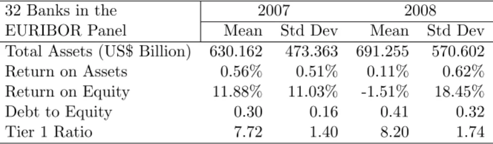
Table 1: Balance Sheet Variables of the Banks in the Sample
32 Banks in the 2007 2008
EURIBOR Panel Mean Std Dev Mean Std Dev
Total Assets (US$ Billion) 630.162 473.363 691.255 570.602
Return on Assets 0.56% 0.51% 0.11% 0.62%
Return on Equity 11.88% 11.03% -1.51% 18.45%
Debt to Equity 0.30 0.16 0.41 0.32
Tier 1 Ratio 7.72 1.40 8.20 1.74
in our restricted sample, we gathered additional data on total assets, return on assets, return on
equity, debt to equity ratio and Tier 1 Capital ratio. Table 1 shows descriptive statistics of these
variables, providing a broad picture of the size and performance of the banks in our final sample.
As additional measures of credit risk, we collected data from Markit on spreads of five-year senior
Credit Default Swaps (CDS) referenced to banks’ bonds. Also, for a subset of these 32 banks that
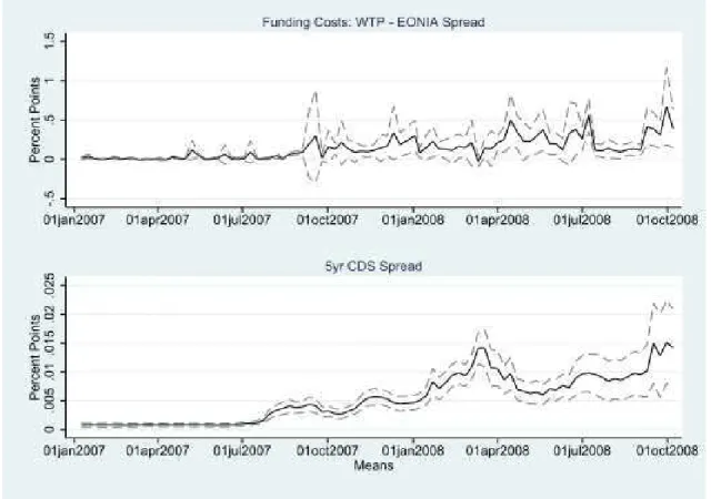
are publicly traded, we have data on market capitalization from Bloomberg. In Figure 1, we plot
the average willingness-to-pay - EONIA spread, and the average CDS spread for the banks in the
sample. We include one standard deviation bands to indicate the dispersion of these measures
across banks.
We also use reports of the European Commission on government interventions in individual
banks (EC 2011). For 629 banks that appear in the liquidity auctions from 2007 and 2008, we
identified 20 banks that received targeted government support at least once. Eight of them belong
to the group of 32 banks in the restricted sample. On top of these targeted ones, there were
also numerous non-targeted bailouts in which various governments helped multiple or all of the
banks in their respective countries. Table 2 shows that 50% of these banks in fact received help
in multiple rounds. The most notorious recepients of government funds were the Anglo Irish Bank
Corporation, which was eventually nationalized, and the IKB Deutsche Industriebank, which after
a generous government injection was almost fully privatized in August 2008. From the other 18
banks, 1 more is from Ireland, 8 are German, 2 are from Austria, Belgium and Netherlands, and 1
bank comes from France, Greece and Slovenia. The bailouts can be categorized into several waves.
The first wave, which included 5 bailouts, occurred before the collapse of Lehman Brothers between
Figure 1: Average Willingness-to-Pay and CDS Spreads for the Banks in the Sample (one standard deviation bands included)
mechanism from auctions to fixed rate tenders the second wave followed with 14 bailouts before
May 2009. Later, there were additional 17 bailouts before July 2011.
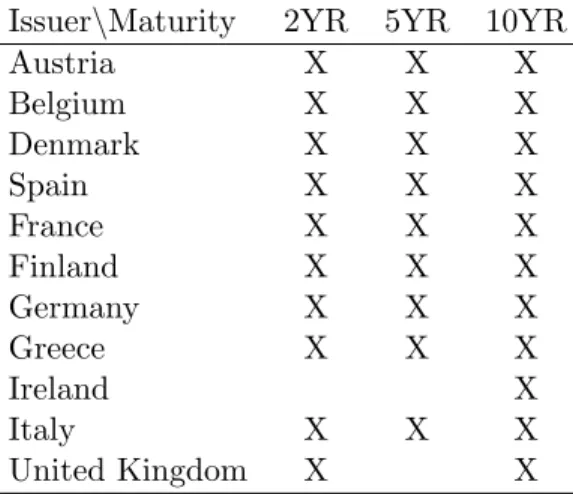
In order to control for common sources of variation in the bank’s funding costs, we also gathered
data from Thomson Reuters’ Datastream on government bonds yields, at different maturities, for
eleven European countries. In total, we have 30 series of the yield to maturity (YTM) of government
bonds for the relevant time range (January 2007 - October 2008). Table 3 lists all these bonds by
issuer and maturity.
We now move on to discuss how to link our model and these data to get at a measure of systemic
Table 2: Data Summary: Bailouts
Summary Statistics of Bailouts
# of Bailouts # of Banks Average Size (in mile)
0 609
1 10 3,327
2 7 18,397
3 1 4,425
4 1 5,825
5 0
6 1 7,359
Table 3: List of All Bonds Included as Controls in the Estimation
Issuer\Maturity 2YR 5YR 10YR
Austria X X X
Belgium X X X
Denmark X X X
Spain X X X
France X X X
Finland X X X
Germany X X X
Greece X X X
Ireland X
Italy X X X
United Kingdom X X
We obtained data on bonds yield-to-maturity from Thomson Reuters’ Datastream.
4
Estimation
We proceed in two steps. First, we use the equilibrium model of bidding in a discriminatory auction
described above to link the bids in the liquidity auctions to the implied willingness-to-pay for repo
loans or, equivalently, to the opportunity funding costs. As we described in Cassola et al. (2013)
this measure provides us with information on prices (interest rates) that a given bank would have
to pay to secure liquidity from other sources on the interbank market. Since there likely are various
important factors which affect the evolution of banks’ funding costs from week to week, and which
are unobserved to the econometrician, we will use an estimation method which uses data only from
network structure that is consistent with the correlation patterns. We then propose our measure
of systemic risk, which is based on this estimated network structure.
4.1 Estimation of the Cost of Funding
Since this method is discussed in detail in Cassola et al. (2013), we describe it here only briefly.
Equation (1) provides us with the link between the observable data (bids) and the variables of
interest: banks’ funding costs. This inversion of bids is a common approach in the empirical
auction literature at least since Guerre, Perrigne and Vuong (2000). In order to invert bids using
equation (1) we need to estimate the distribution of the market clearing price,Pc, which is
bidder-specific, because it depends on the submitted bid.
To do that we employ the resampling method introduced in Horta¸csu and McAdams (2010) and
further developed in Kastl (2011) and Horta¸csu and Kastl (2012). In order to perform this step
we impose the assumption of independence and ex-ante (within group) symmetry among banks
(within one of M groups). The resampling procedure allows us to simulate the distribution of
market clearing price using bids submitted only within one particular auction. By repeatedly
drawing with replacementNm−1 andN−m bids from the observed sample, we can simulate a state of the world, a particular realization of the residual supply from the perspective of a bank from
group m. This simulated residual supply intersected with the submitted bid delivers a particular
realization of the market clearing price potentially faced by this bank. Repeating this procedure
for each bank in each auction yields an empirical distribution of the market clearing prices and
thus allows us to evaluate the probabilities in equation (1). In Cassola et al. (2013) we showed that
with uncertainty about the available supply our estimator is consistent as the number of bidders
within an auction goes to infinity.
We use this method to estimate the willingness-to-pay of each bank that participates in a
given auction. Since most banks participate quite frequently (and the major ones participate
virtually always), we thus obtain a time series of (opportunity) funding costs for every bank, which
4.2 Estimating the Network of Spillovers using he Adaptive Elastic Net
In order to explicitly define what we mean by systemic risk, consider the following simple model of
the dynamics of the cost of funding:
vi,t =β0,i+
X
j
βi,jvj,t−1+XtT−1γi+ǫi,t (2)
wherevi,tis the cost of funding of bankiin periodt, andXtis a vector of controls intended to reflect
aggregate “common” shocks (in practice, we use sovereign bond yields at different maturities). The
cross-effect, βi,j, captures the impact of a shock toj’s cost of funding, such as a negative shock to
its portfolio, on i’s funding costs. A possible channel through which this effect might operate is
the exposure of other banks toj’s bonds, which are likely to loose value following a negative shock
due to j’s increased probability of default. Another possible mechanism linking banks funding
costs are asset fire-sales, where the sale of a large quantity of assets by one bank in order to meet
capital requirements leads to a devaluation of other banks’ asset portfolios, as in Greenwood et al.
(2015). AssumingXt adequately controls for common shocks, theβi,j’s could be interpreted as the
effect due to direct debt contracts between banks or fire-sale spillovers. In Section 5.4-5.6 and the
Appendix A.2-A.3, we conduct several robustness exercises, including an instrumental variables
strategy.
4.3 Estimation Procedure: The Adaptive Elastic Net
A first important challenge in interpreting a specification like (2) from a causal perspective is the
presence of omitted sources of correlation betweenvt−1andvt(the vector of all banks’ funding costs att−1 andt, respectively). We attempt to address this issue by adding a number of controls inXt
to account for common shocks. Coupled with the large number of banks in the system (who can
all, in principle, be on the right hand side of the regression) this creates yet another challenge, that
there are more parameters to estimate than the number of time series observations per bank. For
the time being we will assume the vector Xt is given and will now discuss some technical aspects
To deal with the “too many covariates” problem, we use theelastic net method of Zou and Hastie
(2005), which is a mixture of a Ridge Regression with the Least Absolute Shrinkage and Selection
Operator (LASSO) (Tibshirani 1996). For simplicity, consider the classical linear regression model
y=Zθ+u, where the sizes ofy andZ areS×1 andS×N, respectively. The adaptive elastic net
estimator of this model can be defined as:
ˆ θenet =
1 +λ
2(1−αe) argminθ∈Θ k
y−Zθk22+λ
(1−αe)
2 kθk
2
2+αekθk1
(3)
wherek·k1 and k·k2 denote theL1 andL2 norms, respectively. The term 1 +λ
2(1−αe)
is a bias
correction factor added by Zou and Hastie (2005) to lessen the downward bias due to double
penalization.
For a given sample, the estimates ˆθenet are a function of the penalty parameters λ and αe.
The two extreme cases are LASSO (αe= 1) and Ridge regression (αe= 0). When the L1-penalty
(LASSO) is sufficiently large, some of the coefficients will be exactly zero, selecting a subset of all
possible regressors. This property makes the LASSO particularly suitable for model selection in
applications where the researcher has strong reasons to believe that some of the variables in the
regression do not belong to the true model generating the data. In our case, this is equivalent to
assuming that the network of interbank links is sparse. Moreover, the LASSO can be modified to
select the right model consistently, as shown by (Zou 2006). This can be achieved by employing
the “adaptive LASSO” which includes adaptive weights to penalize each coefficient differently in
the L1 penalty. The adaptive LASSO also has the oracle property, i.e., it performs as well as an
estimator that only includes the variables in the true underlying model, in terms of the convergence
rate of the non-zero coefficients.
However, consistent model selection is not our only concern. It is a well known fact that the
LASSO does not perform well when (some of) the RHS variables are highly correlated. This problem
is of particular relevance to our application, since it is almost by definition of the financial network
that the funding costs will be contemporaneously correlated. Zou and Hastie (2005) proposed the
elastic net estimator in (3) precisely to deal with this issue.5 Unlike the basic LASSO, the elastic
5
net can select groups of strongly correlated predictors, improving the prediction accuracy of the
LASSO. Moreover, the elastic net can also be slightly modified to guarantee that the oracle property
holds. In fact, theadaptive elastic net of Zou and Zhang (2009) combines the weightedL1 penalty
of the adaptive LASSO with theL2 penalty included in elastic net and it inherits the advantages of
both methods over the LASSO. It has the oracle property, as adaptive LASSO does, and handles
highly correlated covariates, as elastic net does. The adaptive weights in theL1 penalty are given
by ˆwj =
θˆenet,j
−δ
, whereδ is a positive constant. Given those weights, the adaptive elastic net
estimates are:
ˆ θanet=
1 +λ
2(1−αe)
argmin
θ∈Θ k
y−Zθk22+λ
(1−αe)
2 kθk
2
2+αe
N
X
j=1
ˆ wj|θj|
(4)
where an infinite weight ( ˆwj = ∞) implies that the j−th variable is not selected (ˆθj = 0). We
choose the adaptive elastic net as our estimation procedure, because it has the desired properties
just mentioned, but also because it allows for consistent estimation of the distributions of the
corresponding estimators by means of the bootstrap, as shown by Chatterjee and Lahiri (2013).6
There are two penalty parameters in the adaptive elastic net: αe and λ. To perform the
estimation, we fix αe = 0.5 and then we use cross validation to find the optimal λ. We use the
procedure just described to independently estimate (2) for each bank. Our main focus of interest is
the resulting estimate ofB, the matrix of direct spillover effects. Our measures of systemicness and
vulnerability rely on such estimation. In Appendix A.2 we perform a robustness check to assess the
sensitivity of the results to changes in αe. For αe ∈ {0.1,0.5,0.9} the results are all qualitatively
very similar. Besides the sparse “prior” implicit when choosing a LASSO-type estimator, we restrict
the estimates ˆθanet to be non-negative by letting Θ = RN+ in (3) and (4), since our focus are the
negative externalities that result from an increase in the funding costs of individual banks. We have
estimated the model without imposing the non-negativity constraints and only a few parameters
take negative values.
the presence of correlated RHS variables.
6As a robustness check on the sensitivity of the results to variation in the individual weights in the adaptive Lasso
There is very active current literature in statistics and econometrics dealing with inference for
these type of estimators. To obtain confidence intervals for our estimates, we apply a refinement
of bootstrap proposed by Chatterjee and Lahiri (2013) described in section A.5 in the appendix.
4.4 Systemic Risk and Network Centrality
Equation (2) can be rewritten in matrix form as
vt=β0+BTvt−1+ηt, ηt= ΓXt+ǫt (5)
By assumption, B represents the network of one period-ahead spillover effects between banks, as
captured by the lagged correlations between their cost of funding. Borrowing some terminology
from Network Analysis,B is (the matrix representation of) a weighted directed graph (a network),
Bi,j is the weight of the link from bank ito bank j, and Bi,j = 0 indicates that there is no such
link. Our measures of systemicness and vulnerability are entirely based on the properties of the
matrix B. Since they are closely related to centrality measures from the networks literature, we
will briefly review the latter before introducing these two concepts.
For a given node iin a networkB, its “Katz centrality” is defined as:
kci(a) =
∞
X
s=1
N
X
j=1
as(Bs)i,j (6)
where the parameter a is positive and lower than the reciprocal of the largest eigenvalue ofB, in
absolute value, to guarantee convergence. Notice further that kc
i(a) is the i-th component of the
vector:
kc(a) =(I −aB)−1−I1 (7)
where1is a vector of ones. Katz centrality calculates the relative importance of a node within the
network by including the sum of its links (the number of direct neighbors in a binary graph) as well
as the weighted sum of the links of its indirect neighbors (those to which the node is connected only
through links with other nodes). If a <1, the weight assigned to the indirect neighbors decreases
A clear benefit from our reduced form specification (2) is that it provides a straightforward
inter-pretation of Katz centrality in terms of total effects of idiosyncratic shocks. Assuming stationarity,
(5) can be iterated forward to obtain:
vt+s = s
X
τ=1
BTτ
β0+ BT
τ
vt−1+
s
X
τ=0
BTs−τ
ηt+τ (8)
Letǫi,t = 1 andǫi,t+1+s =ǫj,t+s= 0 for all j and all s≥0. Conditioning on the realized values of
Xt+s, the response in the WTPs of all banks to this shock is given by:
∆vt+s= s
X
τ=0
BTs−τ
ǫt+τ = BT
s
ǫt (9)
Now, if K = P∞
s=1Bs = (I−B)−1 −I, then Ki,j can be interpreted as the long run effect of a permanent shock of 100bp toi′sfunding costs onj′sfunding costs (orM A(∞) representation of the specified AR(1) process). Moreover, the parameterain (7) can be used to assign lower weights to
more distant responses in the funding costs. We usea= 0.9 since at our estimated network matrix,
the shocks then completely dissipate after two years, which seems like a reasonably conservative
upper bound. We therefore use the Katz centrality measure to define the following notions of
systemicness (as the average total effect of a shock to bank i’s funding costs on the funding costs
of a bank in the network):
kis(a) = 1 N
∞
X
s=1
N
X
j=1
as(Bs)i,j (10)
and vulnerability (as the average total effect on bank i’s funding cost of a shock to the funding
costs of a bank in the network):
kiv(a) = 1 N
∞
X
s=1
N
X
j=1
as(Bs)j,i (11)
where the difference between the two measures is whether we use the matrix B directly or its
4.5 Controlling for common shocks
As already mentioned, one important concern with the reduced form specification (5) is the
exis-tence of exogenous common components that might be driving the correlation between vt−1 and
vt. For instance, there could be a common trend in all the funding costs in the vectorvt, and then
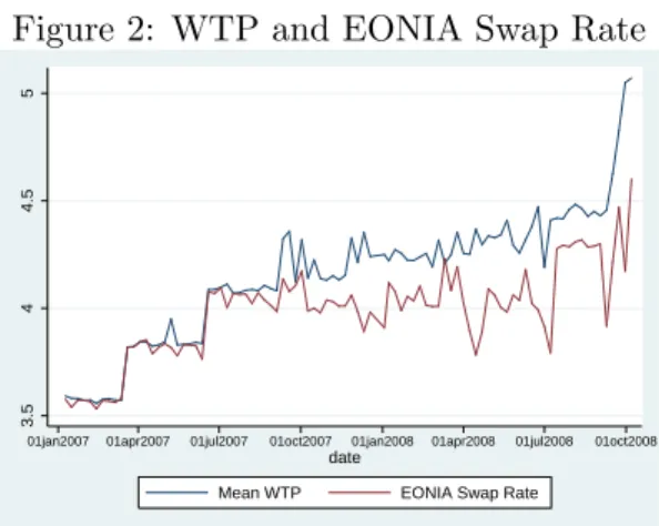
the recovered correlations between vi,t−1 and vj,t would overestimate the actual spillover effect. To control for the expectations of the market rates, our main variable of interest is the spread
between the funding costs and the EOINA swap rate. In fact, adjusting for EONIA accounts for a
large share of the common trend in the vi,t’s, specially before August 2007, as shown in figure 2.
Without adding any other controls, a positive estimate of βi,j in (2) implies that a positive shock
to bank j’s funding costs spread over EONIA is associated with an increase in the funding costs
spread for banki, one period ahead.
Figure 2: WTP and EONIA Swap Rate
3.5
4
4.5
5
01jan2007 01apr2007 01jul2007 01oct2007 01jan2008 01apr2008 01jul2008 01oct2008
date
Mean WTP EONIA Swap Rate
As further controls for omitted common shocks, we also gathered data from Thomson Reuters’
Datastream on government bonds yields at different maturities for ten European countries. In
total, we have 30 series of the yield to maturity (YTM) of government bonds for the relevant time
range (January 2007 - October 2008). Let Xc,m,t = log (Rc,m,t−1)−log (Rc,m,t−2), whereRc,m,t is the (annualized) YTM of a bond from government c with maturity m at time t. The vector Xt
in (2) is the collection of all 30 Xc,m,t’s. We include these lagged differences in government bond
yields as regressors to control for possible sources of covariation of the funding costs.7 First, it
7
is highly likely that most banks in our sample hold portfolios of sovereign bonds, so they should
be commonly exposed to variation in their prices, albeit to different degree. Second, the bond
yields could be interpreted as proxies for general macroeconomic conditions in the country issuing
the bond. In fact, such yields include risk premia that reflect market expectations on the state
of the respective economies. Banks in the same country may be affected by country-level shocks
that could be at least partially captured by the variation in bond yields. An important caveat is
that prices might decrease due to firesales that result from liquidity or credit tightening conditions
(as in Greenwood et al. (2015)). Moreover, banks might be using the bonds as collateral in the
repo market, hence price volatility would directly imply an increase in their cost of funding as the
quality of their collateral would deteriorate. This may trigger bond liquidations and deleveraging
that would increase the price volatility and deteriorate the collateral even further. Thus controlling
for bond yields, which are inversely related to their prices, could prevent such firesales from being
captured, as a propagation channel, in the estimated residual comovements of the funding costs.
5
Results
5.1 Systemic Risk
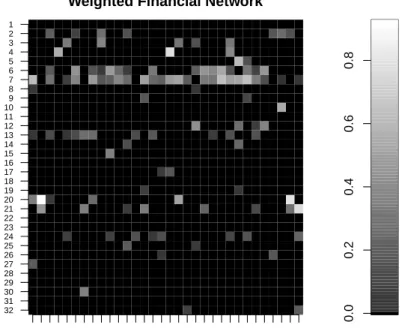
Figure 3 illustrates the results of one specification of our model of the financial network. Thei-th
column corresponds to the regression of vi,t on the vector vt−1. The lighter squares correspond
to the variables that are selected by the LASSO component of the elastic net estimation of such
regression. The lighter the color, the stronger the effect. More generally, the light squares can be
interpreted as positive effects of one-period lagged funding costs of the row (y-axis) bank on the
column (x-axis) bank’s funding costs. It is evident that shocks to some banks affect a large number
of their rivals. The number of lighter squares in a row corresponds to the number of (direct) links
starting from that bank in the financial network. This number, the degree of the corresponding
node in the binary counterpart of this matrix, is one measure of network centrality, but it ignores
information on the strength of these links (their weight). The definition of degree can be easily
generalized to include such information. We could compute the degree of a node as the sum of
not only takes the strength of the direct links into account, but also uses the information on the
(indirect) paths captured by the powers of the matrix representing the directed weighted network.
Weighted Financial Network
1 3 5 7 9 11 13 15 17 19 21 23 25 27 29 31 32
31 30 29 28 27 26 25 24 23 22 21 20 19 18 17 16 15 14 13 12 11 10 9 8 7 6 5 4 3 2 1
0.0
0.2
0.4
0.6
0.8
Figure 3: Elastic Net Coefficients: (1st order) Effect of a Shock to Row Bank’s (lagged) Funding Costs on Column Bank’s Funding Costs.
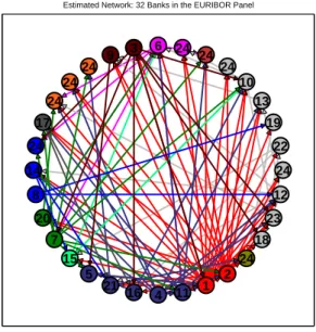
In Figure 4 we plot the estimated financial network. For confidentiality reasons, we cannot
report the names of the banks. Each depicted node corresponds to a bank that is a member of the
EURIBOR panel. The arrows between them correspond to positive coefficients in the respective
adaptive elastic net regression. More precisely, there is an arrow from bankito bankj if banki’s
lagged cost of funding is correlated with bank j’s cost of funding. Different colors correspond to
different countries. Finally, the number in each node corresponds to the systemic rank of that node
according to the Katz centrality measure (fora= 0.9). Even though the strength of the links is an
important component in the centrality ranking, it is also the case that the top ranked banks have
many links connecting them directly to other banks, as it is clearly the case for the two highest
ranked banks.
Tables 4 and 5 offer a quantitative assessment of our estimates (see section A.5 for confidence
Estimated Network: 32 Banks in the EURIBOR Panel
6 24
24 24
10 13
19
22
24
12
23
18 24 2 1 11 4 16 21 5 15 7 20 8 14 24 17
24 24
24 9
3
Figure 4: Financial Network
Table 4: First order effect of a 100bp shock to each of the top 5 systemic banks on all banks (Country means reported)
AT BE DE DK ES FR GR IE IT JP NL UK
Spanish Bank (ES) 0.0650 0.5135 0.3367 0.2185 0.1847 0.2886 0.5260 0.2342 0.0236 0.1723 0.3130 0.2730 Spanish Bank (ES) 0.3309 0.0000 0.1527 0.0000 0.2164 0.0989 0.0000 0.0751 0.0000 0.0397 0.1295 0.4565 British Bank (UK) 0.0000 0.0000 0.1025 0.0000 0.1754 0.0692 0.0000 0.2264 0.0921 0.0000 0.0000 0.1161 French Bank (FR) 0.0000 0.0000 0.0530 0.0000 0.1958 0.0469 0.0000 0.1323 0.0104 0.0000 0.0248 0.0000 French Bank (FR) 0.0000 0.0000 0.0000 0.0000 0.1788 0.0000 0.0000 0.0000 0.0000 0.0000 0.0000 0.0000
net regression of the funding costs of the five most systemic banks, i.e., the coefficients ofB from
equation (2), where we aggregated these effects to the country level. While these coefficients still
need to be interpreted with caution (due to omitted variables and other potential confounding
factors), we believe that they offer an interesting perspective. For example, all five top ranked
banks seem to impact the funding costs of Spanish banks, and one Spanish bank has a large effect
on the funding costs of Belgian and Greek banks. If all top 5 banks suffered an increase in their
funding costs of 100 basis points, the average funding costs of Spanish banks would rise right away
by more than 95 basis points. By contrast, Italian banks do not seem to react right after the shock,
the direct impacts are all below 10bp. However, this does not mean that they are not exposed to
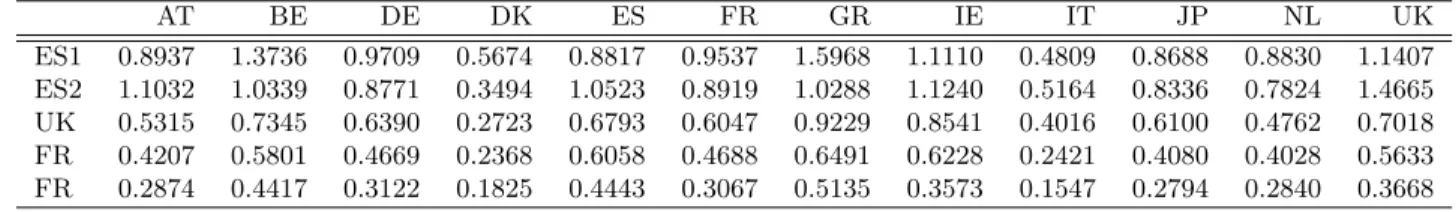
Table 5: Total effect of a 100bp shock to each of the top 5 systemic banks on all banks (Country means reported)
AT BE DE DK ES FR GR IE IT JP NL UK
ES1 0.8937 1.3736 0.9709 0.5674 0.8817 0.9537 1.5968 1.1110 0.4809 0.8688 0.8830 1.1407
ES2 1.1032 1.0339 0.8771 0.3494 1.0523 0.8919 1.0288 1.1240 0.5164 0.8336 0.7824 1.4665
UK 0.5315 0.7345 0.6390 0.2723 0.6793 0.6047 0.9229 0.8541 0.4016 0.6100 0.4762 0.7018
FR 0.4207 0.5801 0.4669 0.2368 0.6058 0.4688 0.6491 0.6228 0.2421 0.4080 0.4028 0.5633
FR 0.2874 0.4417 0.3122 0.1825 0.4443 0.3067 0.5135 0.3573 0.1547 0.2794 0.2840 0.3668
a
Averages across banks within a country reported.
bThe total effect is computed using the Katz centrality measure with
α= 0.9.
Table 5 reports the total effect, i.e., not only the first order effect reported in Table 4, but
also the feedback from indirect effects and persistence captured by all the powers ofB in the Katz
centrality measure. Comparing the magnitudes across the two tables, the amplification of the
shocks due to feedback seems quite high. The total effect of a 100bp shock to the funding costs
of any of these top five systemic banks on banks in other countries is, in many cases, larger in
magnitude than the original shock. This holds, in particular, for the two most systemic Spanish
banks. Notice further than when the total effects are accounted for, the Italian banks are similarly
exposed to contagion as banks in other regions. Still, Italian and Danish banks seem to be, on
average, the less vulnerable to contagion from the most systemic banks.
We investigate the relative importance of intra-country effects further by highlighting the links in
the network that connect two banks in the same country. Heuristically, by means of such comparison
we want to test the hypothesis that a large share of systemic risk is due to the effect that the increase
in a bank’s cost of funding has on the costs of funding of other banks in its own country of origin.
Figure 5 displays the binary directed graph (ignoring the weights), highlighting the intra-country
links. Clearly, most of the links in the network connect banks in different countries. Moreover, on
average the within country links account for no more than 9% of the average direct (first order)
effect of a 100bp shock to the cost of funding of the banks in our sample. 8
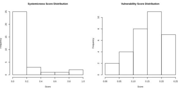
In Figure 6 (left panel) we plot the histogram of our systemicness measure: the average total
effect on a rival when a bank suffers a 100 basis point increase in its cost of funding. Our results
8
Intra−Country Subsets of the Network
AT BE DE DE DE DE DK ES FR FR GR IE IT JP NL UK UK UKNL NL NL JP IT IT IT IE IE GRFR FR FR FR FR ES ES DK DE DE DE DE DE DE DE DE DE BE AT AT
Estimated Network: 32 Banks in the EURIBOR Panel
AT:6 AT:24 BE:24 DE:24 DE:10 DE:13 DE:19 DE:22 DE:24 DE:12 DE:23 DE:18 DK:24 ES:2 ES:1 FR:11 FR:4 FR:16 FR:21 FR:5 GR:15 IE:7 IE:20 IT:8 IT:14 IT:24 JP:17 NL:24 NL:24 NL:24 UK:9 UK:3
Figure 5: Relative importance of intra-country effects: In the left panel the links between two banks from the same country are highlighted in white. In the right panel, each number is the systemicness ranking of the respective node.
suggest a fair amount of heterogeneity of the impact of such a shock to a bank’s funding costs.
While a shock to many banks in the EURO zone would not imply any substantial change in the
funding costs of its rivals, there are a few important exceptions. In particular, there are two banks
in the EURIBOR panel such that if they were to face a permanent 100 basis point increase in
its funding costs, on average the funding costs of the other banks could increase by as much as
approximately 90 basis points. We also plot, in the right panel, the histogram of the average total
effect on each bank when a rival suffers a 100 basis point increase in its cost of funding. Clearly,
the distribution is much less skewed, with most of the banks experiencing an average increase in
their funding cost between 15 and 20 basis points.
5.2 Network Structure
If the weights on the links are ignored the network of spillover effects can be represented as a
directed graph. That is, a link or edge from bank i to bank j represents a positive correlation
between bank i’s lagged funding costs and bank j’s funding costs. Moreover, if the direction of
Systemicness Score Distribution
Score
Frequency
0.0 0.2 0.4 0.6 0.8 1.0
0
5
10
15
20
25
Vulnerability Score Distribution
Score
Frequency
0.00 0.05 0.10 0.15 0.20 0.25
0
2
4
6
8
10
Figure 6: Katz Centrality Distribution. Left: Average total effect on a rival of a 100bp shock to the funding costs of each bank in the sample. Right: Average effect on the funding cost of each bank of a 100bp shock to the funding cost of a rival.
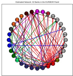
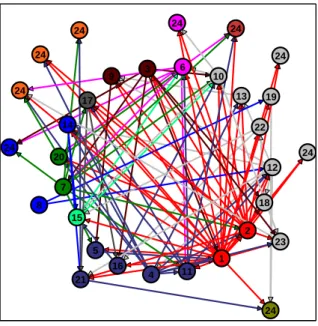
banks represents that either of them is connected to the other one. As can be seen directly by
inspecting Figure 7, the undirected graph has only one (connected) component, meaning that there
is no subset of banks completely isolated from the rest of the network. Figure 7 also illustrates
other salient features of the network. The outer circle, formed by all banks labeled ‘24’ (the lowest
position in the systemicness ranking), contains all the banks that have no outgoing edges, that is,
there is no edge from these banks to any other bank in the network. However, there are several
edges from other banks to all of the banks in the outer circle. Therefore, such banks are exposed to
contagion if another bank in the network suffers a shock to its funding costs, but they do not impose
any significant risk to any other bank (they do not relay the shocks further). If the main driver of
correlation among bank’s funding costs were interbank lending, then such network structure would
suggest that around a quarter of the banks in our sample behave as net lenders within the network,
which exposes them to counterparty risk. In contrast, banks in the inner circle form a strongly
connected component, which means that there is a path (sequence of outgoing edges) from each
to any other of them. Furthermore, there is a path from all banks in the inner circle to all other
from this subset of roughly two thirds of the banks in our sample.
Figure 7: Network Structure. All banks are labeled according to their systemicness ranking and their color correspond to their country of origin as in figure 5. The outer circle (all banks labeled ‘24’) is formed by banks that have no outgoing edges. The inner circle is a strongly connected component, that is, there is a path (a sequence of outgoing edges) from all these banks to each other.
Estimated Network: 32 Banks in the EURIBOR Panel
6 24
24
24
10
13 19
22
24 12
23 18
24 2
1 11 4 16 21
5 15 7 20
8 14
24
17 24
24 24
9 3
Similar results have been found both in the theoretical and the empirical literature. Farboodi
(2014) develops a model of the interbank lending market with endogenous network formation. Her
model predicts a ‘core-periphery’ network structure9, where a subset of the banks (the periphery)
provides funds to another set of highly interconnected banks (the core) that act as intermediaries
and/or invest those funds. Even though we are focusing on a sample of substantially large banks,
all of which presumably have profitable investment opportunities, it is worth noting that a similar
structure arises.
Bech and Atalay (2008) analyse the federal funds market as a network, where an edge from
bank i to bank j means that j borrows fed funds overnight from i. They find that many of the
largest banks in the US (in total assets) form a strongly connected component (around 10% of the
9
almost 500 banks in their sample). Also, most of the small banks (roughly 58% of all the sample
in 2006) are net lenders to banks in the first group. Even though, according to our estimates
around 60% of the banks in the Euribor panel belong to the strongly connected component, there
is some resemblance between our results and those in Bech and Atalay (2008). Again, we are only
considering a subset of the largest banks bidding for funds at the ECB (all of whom belong to the
Euribor panel) so it is consistent with what these authors find that most banks in our sample are
exposed to each other. What is surprising is that even among these large banks, we find some that
are exposed to, but do not expose others to contagion.
Wetherilt et al. (2010) study the network structure of the unsecured overnight loan market in the
UK during 2006-2008. Noteworthily, there are only a few (12 to 13) banks trading through CHAPS
(the British Clearing House Automated Payment System) and many of them are also included in
our sample. These authors also describe what they find as a ‘core-periphery’ network structure.
Roughly speaking, they too define the core as a subset of highly interconnected banks. Moreover,
they observe that the size of the core increased as the crisis unfolded. However, in contrast with our
results and those in the literature previously mentioned, they find that banks in the periphery both
borrow from, and lend to, banks in the core. Nevertheless, their definitions of ‘core’ and ‘periphery’
are based on the likelihood that there is an edge (an overnight loan) connecting two banks in each
group and not on a partition of the set of nodes induced by strongly connected components. The
takeaway is that, despite the differences in how these sets are defined, banks seem to naturally
divide into two groups, depending on how tightly or loosely connected they are to each other, and
such result seems to hold even when just a small number of large banks is considered.
Based on simulations, Elliot et al. (2014) make an interesting prediction about contagion effects
in a network with a related ‘core-periphery’ structure. If the level of integration (roughly, how
much of a bank’s assets is owed to its counterparties) among core banks is low, then the failure of
any bank is not likely to generate wide-spread contagion. As integration rises to middle levels, the
number of institutions that fail as a consequence of the initial failure also rises. Finally, for high
levels of integration among core banks, the results depend on whether the bank that suffers the
a result is weakly higher than for middle-sized integration. However, if it belongs to the periphery,
the effect is non-monotonic and the number of failing banks decreases. It is tempting to apply such
results to our estimated network to try to predict how exposed to contagion the whole system is.
However, there are some prominent differences between the network structures that prevents us
from doing so. First, we identify a set of banks that have no outgoing edges (the outer circle in
figure 7). Thus, if any of them where to fail (in our model that would be a shock to its funding
cost beyond some healthy threshold), our estimates would predict no further failures, regardless
of the level of integration. Second, in Elliot et al. (2014) the core of the simulated network is a
clique, that is, a set of banks that are completely connected (no missing edges between them). In
contrast, we estimate quite a sparse network, and even within the strongly connected component
(the inner circle in figure 7) there are a lot of missing edges (as a matter of fact, only 20.5% of all
possible edges in such set belong to the network).
5.3 Vulnerability and Bailouts
Eight out of 32 banks in our sample received targeted government support after August 2007 (most
of them after October 2008, that is, out of sample). We run probit regressions of the probability
of receiving such support (a bailout) on vulnerability (Vuln score), Return on Assets (ROA2008),
Return on Equity (ROE2008), Tier 1 Capital Ratio, a measure of leverage (Debt to equity 2008)
and Average CDS spread of Dec. 2008 (cds dic). The results are reported in Table 6. Notice
that the coefficient on Vulnerability Score has the expected sign and is significant in all regressions.
ROA and ROE are also significant, but Tier 1 Ratio, Debt to Equity2008, and CDS spread are not.
Therefore, our measure of vulnerability does a better job at predicting bailouts than CDS spreads,
Tier 1 Capital and leverage. Our findings regarding Tier 1 Ratio, ROA and ROE are consistent
with analogous results recently reported by the European Systemic Risk Board in Alves, Ferrari,
Franchini, Heam, Jurca, Langfield, Laviola, Liedorp, Snchez, Tavolaro and Vuillemey (2013).
We compare our vulnerability score with analogous measures of exposure to contagion based on
Euribor quotes, CDS spreads, market capitalization and CoVaR (Adrian and Brunnermeier (2011)),
in terms of their ability to predict bailouts.10 As a benchmark, we use model (4) in Table 6, because
10
I(Bailout)
(1) (2) (3) (4) (5)
Vuln score 0.487∗ 0.457∗ 0.522∗ 0.560∗ 0.541∗
(2.23) (2.22) (2.00) (2.12) (2.12)
ROA2008 -1.626∗ -1.745∗
(-2.68) (-2.56)
Debt to Equity2008 -0.402 -0.0904 -0.496 -0.312
(-0.41) (-0.09) (-0.50) (-0.30)
ROE2008 -0.0460∗ -0.0540∗ -0.0522∗
(-2.71) (-2.71) (-2.76)
Tier 1 Ratio 0.0926 0.132 0.127
(0.48) (0.70) (0.67)
CDS -19.78 -41.47 -37.61
(-0.35) (-0.76) (-0.70)
Const. -2.979∗ -3.126∗ -3.588∗ -4.059∗ -4.102∗
(-2.54) (-2.67) (-1.98) (-2.18) (-2.19)
N 32 32 32 32 32
tstatistics in parentheses
+
p <0.10,∗
p <0.05
Table 6: Probit Models for the Probability of a Bailout. For model (4), the average marginal effect of a 1bp increase in the vulnerability score on the probability of a bailout is (an increase of) 3.7 percentage points, and the marginal effect for the average bank is 4.4 percentage points.
that is the specification of the probit that includes the most relevant set of controls. We report the
results in Table 7, where each column corresponds to a different vulnerability measure included
as a covariate (all the other controls are the same as in model (4) in Table 6). As opposed to our
vulnerability score, we find that none of these alternative measures significantly predict bailouts at
the 5% level. However, the measures based on market capitalization and CoVaR are still significant
at the 10% level. In this last two cases, though, the regressions only include the subset of banks in
I(Bailout)
Vulnerability Euribor CDS Market Cap. Covar
0.462 0.121 0.958+ 79.91+
(0.474) (0.724) (0.507) (48.33)
N 32 32 23 23
Standard errors in parentheses
+
p <0.10,∗
p <0.05
Table 7: Probit Models for the Probability of a Bailout Using Alternative Proxies for Funding Costs. All the columns correspond to model (4) in Table 6, when the vulnerability score is replaced by alternative measures of exposure to contagion that are not based in our estimates of Banks’ funding costs.
5.4 Controlling for Common Shocks
In general terms, we found evidence that the scores and rankings are robust to the inclusion of
changes in sovereign bond yields as controls in the estimation. Figure 8 shows the corresponding
systemicness and vulnerability scores and rankings. Clearly, most of the changes in the estimates
due to controlling for bond yields are minor. This is a direct consequence of the fact that only
a few bonds, or in some cases none of them, are selected by the elastic net in the regression for
each bank’s funding costs. That is, our estimates suggest that the lagged funding costs of the
counterparties are a stronger determinant of the funding costs of a bank than the returns on any
portfolio of sovereign bonds. Still, the score of the most systemic bank is reduced by 21 basis
points when the controls are included, which is not a negligible difference. That is, not including
the proper controls would, at the very least, result in an overestimation of the risk that the most
systemic bank represents to the system as a whole.
5.5 Alternative Measures of the Cost of Funding: Euribor Quotes and Bids
All the banks in our sample belong to the EURIBOR panel and thus they submit daily quotes of
the rate at which they expect a prime bank to lend to another prime bank, through interbank term
deposits, within the euro zone. They also bid in the MROs of the ECB for short-term maturity
funds. Hence, both the Euribor quotes and the quantity weighted bids could in principle be used
5 10 15 20
5
10
15
20
Systemicness Rankings (ρ = 0.98)
Ranking: Bonds as Controls
Ranking: No Controls
0.0 0.2 0.4 0.6 0.8
0.0
0.2
0.4
0.6
0.8
1.0
Systemicness Scores (ρ = 0.98)
Score: Bonds as Controls
Score: No Controls
0 5 10 15 20 25 30
0
5
10
15
20
25
30
Vulnerability Rankings (ρ = 0.99)
Ranking: Bonds as Controls
Ranking: No Controls
0.05 0.10 0.15 0.20
0.05
0.10
0.15
0.20
Vulnerability Scores (ρ = 0.99)
Score: Bonds as Controls
Score: No Controls
Figure 8: Effect on systemicness and vulnerability measures of controlling for government bonds (each point represents a bank in our sample).
vulnerability measures. As mentioned earlier, there are some shortcomings of using such alternative
proxies for the cost of funding faced by banks in the interbank market. Regarding Euribor quotes,
they are self-reported and, as recent scandals unveiled, are likely subject to strategic manipulation
(see, for example, Barclays (2012)). Bids, as we argued earlier, also contain a strategic component.
To assess the effect of this strategic deviations from truthfully revealing their cost of funding, we
compare our systemicness and vulnerability measures (based on the inverted bids from the MROs)
with the ones resulting from estimating network B in equation (5) using monthly averages of the