A Scheduling Method in High-Level Synthesis for RTL Acyclic Partial
Scan Design
Tomoo Inoue
†, Tomokazu Miura
†, Akio Tamura
†, and Hideo Fujiwara
‡†Faculty of Information Sciences, Hiroshima City University
3-4-1 Ozukahigashi, Asaminami, Hiroshima 731-3194, Japan, Ph./Fax:+81-82-830-1575
‡Graduate School of Information Science, Nara Institute of Science and Technology 8916-5 Takayama, Ikoma, Nara 630-0101, Japan, Ph.:+81-743-72-5220, Fax:+81-743-72-5229 {tomoo,tamura}@im.hiroshima-cu.ac.jp, [email protected], [email protected]
Abstract. Acyclic partial scan designis an efficient DFT method. This paper presents a scheduling method for reduc- ing the number of scan registers for acyclic structure. In or- der to estimate the number of scan registers during schedul- ing, we propose provisional binding of operational units, and show a force-directed scheduling algorithm [13] with the provisional binding. Experimental results show that the num- ber of scan registers in the resulting RTL datapaths can be reduced by our method combined with the binding algorithm for acyclic partial scan [12].
Keywords. Acyclic partial scan, high-level synthesis, scheduling, provisional binding.
1 Introduction
Design-for-testability (DFT) at register-transfer level (RTL) is an important approach to the reduction of testing cost. RTL DFT is suitable for today’s VLSI design style — The design modification for testabil- ity is transparent for RTL designers, and the area/delay penalty by the DFT is alleviated by logic synthesis.
Acyclic partial scan design is an efficient DFT method. In this DFT, some of flip-flops in a sequential circuit are replaced by scan flip-flops so that the resul- tant kernel circuit becomes acyclic. Test generation for an acyclic sequential circuit can be performed by ap- plying a combinational test generation algorithm to its time-expansion model[1], and hence a complete test set for an acyclic sequential circuit can be obtained ef- ficiently. Such structure-based DFTs [1]-[4] can be ap- plied to RTL designs since structural properties in RTL designs are generally succeeded to logic level circuits by logic synthesis. An efficient algorithm for finding a minimum set of scan registers that break all feed- back loops in a circuit has been proposed in [5]. Thus,
we can obtain testable circuits with low hardware over- head efficiently.
High-level synthesisrefers to transforming an ab- stract behavioral description into an RTL circuit. Tak- ing DFTs applied to the resultant RTL circuits into ac- count during high-level synthesis, i.e., high-level syn- thesis for testabilitycan reduce the area/delay penalty, and bring out the effect of the RTL DFTs [6]. Many techniques on high-level synthesis for partial scan de- sign have been proposed [7]-[12].
In this paper, we consider a method of high-level synthesis for acyclic partial scan design. High-level synthesis mainly consists of two tasks: scheduling and binding. Takasaki et al. [12] proposed a binding algo- rithm for minimizing the number of scan registers so as to make the kernel acyclic for a given scheduled data flow graph (DFG) or behavior description while keep- ing the area/performance optimality. The experimental results show that the binding method can minimize the number of scan registers for many scheduled DFGs. In this paper, we propose a scheduling method for reduc- ing the number of scan registers for acyclic structure. In order to estimate the number of scan registers during scheduling, we propose provisional binding of opera- tional units, and show a force-directed scheduling al- gorithm [13] with the provisional binding. Experimen- tal results show that the combination of the scheduling algorithm with the provisional binding and the binding algorithm [12] can further reduce the number of scan registers for acyclic structure compared to that of the scheduling algorithm without the provisional binding and the binding algorithm for some example DFGs.
IEEE 2001 Workshop on RTL ATPG & DFT, pp. 7-12, Nov. 2001.
PI
+2 +1
* Const.
+3 PI
+4
PO x
u
v
w d1
y d2
PI
+2 +1
* Const.
+3 PI
+4
PO x
u
v
w d1
y d2
0
1
2
3
4
5 * + +
Const PO
PI
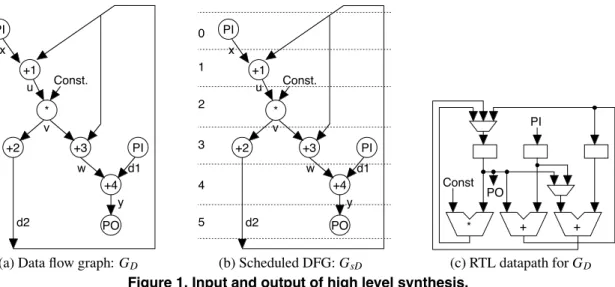
(a) Data flow graph: GD (b) Scheduled DFG: GsD (c) RTL datapath for GD Figure 1. Input and output of high level synthesis.
2 High-Level Synthesis for Acyclic Struc-
ture
2.1 High-level synthesis flow
High-level synthesis (HLS) transforms a behavioral information, which is represented by a data flow graph (DFG) (Fig. 1(a)), into a register-transfer level (RTL) design (Fig. 1(c)). In a DFG, a vertex represents an op- eration with a type (adder, multiplier, and so forth), and an edge represents a variable. Our HLS system derives an optimal RTL datapath in which the number of re- sources (operational units and registers) are minimum for a given DFG with a latency constraint, which is an upper bound of the execution time. In addition, it aims to minimize the number of scan registers required for cycle breaking in the resultant RTL circuits.
HLS mainly consists of two tasks: scheduling and binding. The former, scheduling, is to minimize the upper bound of the number of operational units for each operation type (adder, multiplier, and so on) under a latency constraint by assigning each operation to an appropriate control step. The result of the scheduling is represented by a scheduled DFG (Fig. 1(b)).
The latter binding procedure is further divided into operational unit binding and register binding. Here we consider that operational unit binding is followed by register binding. In these procedures, each opera- tion (variable) in the DFG scheduled by the above pro- cedure is assigned to an operational unit (register) in the resultant RTL datapath, i.e., the binding determines which each operation (variable) shares an operational unit (register) with. As a result, an optimal datapath with minimum numbers of operational units and regis- ters is obtained (Fig. 1(c)).
2.2 Binding algorithm
The optimal operational unit binding problem is re- duced to the minimum clique partitioning problem for a compatibility graph of operations. In a compatibil- ity graph GC(Fig. 2) for a scheduled DFG GsD, a ver- tex corresponds to an operation, and an edge(v1,v2) denotes that operations v1 and v2are compatible, i.e., they can share an identical operation. Note that two op- erations v1, v2 are compatible when they are assigned to different control steps in the scheduled DFG GsD. A clique in compatibility graph GCmeans that all the operations in the clique can share one identical oper- ations, and hence the goal of binding is to partition the compatibility graph with a minimum number of cliques. An efficient heuristic algorithm for the min- imum clique partitioning problem has been proposed [14].
Recall that our goal is to minimize the number of scan registers for acyclic partial scan while minimiz- ing the number of resources under a given latency constraint. In order to take the number of scan reg- isters into account during the above-mentioned mini- mum clique partitioning, by focusing on the fact that sharing may cause a loop, Takasaki et al. [12] repre- sented the strength or possibility of the requirement for scan registers as a weight on an edge in the compati- bility graph, and presented an algorithm for finding a minimum weighted clique partitioning.
In [12], edges(v1,v2) in compatibility graph GCare classified into three cases based on the relation of two operations v1 and v2 in the scheduled DFG GsD, and accordingly edges are weighted as follows1.
1In [12], the weight is specified in more detail according to the scheduled control steps of operations and the number of variables between them. However, we need not such a specified weight in the following discussion, and hence the precise definition is omitted
+2 +1
+3
+4
+2 +1
+3
+4 10
100 100
10 10
(a) Compatibility (b) Minimum weighted graph GC. partitioning. Figure 2. Compatibility graph: GC for adders in GD.
v1and v2are adjacent. The sharing must make a self-loop. A self-loop must need a scan register, and therefore the weight is large.
v1and v2are not adjacent, but reachable. This makes a (global) feedback loop. There must exist at least one scan register on a path between v1 and v2. This, however, implies that an assignment of some variable on the path to a scan register is sufficient. Hence, the weight is relatively small.
There is no path between v1and v2. In this case, no loop is made, and hence the weight is zero.
Based on the above weighting, the weight of a clique is defined as the sum of weights of edges in the clique. A heavy clique is regarded as a sharing that re- quires scan registers strongly. Thus, the problem (min- imizing the number of scan registers with the minimum number of resources) is solved by finding a minimum clique partitioning such that the sum of weights of the cliques is minimum.
Example 1: Fig. 2(a) shows the compatibility graph GC for adders in the scheduled DFG GsD. Fig. 2(b) shows the weights of edges and the optimal clique par- titioning. In this example, large and small weights are given by 100 and 10, respectively, for the simplicity. The number of cliques is two, and hence, the number of adders in the resultant RTL circuits becomes two. The sum of weights of cliques is 10+ 10 = 20, which is the minimum. Note that the weight of any other clique partitioning whose number of cliques is also two is larger than 20 (e.g.,{{+1,+2},{+3,+4}} derives
weight 200). ✷
Similarly, register binding is performed, and thus an optimal RTL datapath can be obtained.
here.
PI
+2 +1Const.
+3 +4
PO 0
1 2
3
4 5
PI PI PI PI
+5 +6
*
Const. –
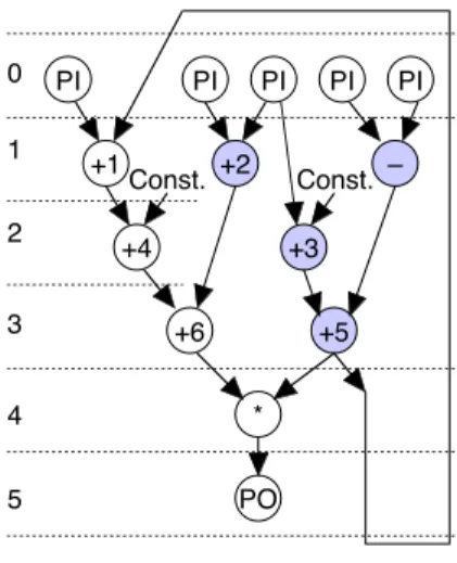
Figure 3. Data flow graph: GD1.
3 Scheduling Algorithm with Provisional
Binding
Recall that the goal of our HLS is to reduce the number of scan registers without obstructing the re- source minimization. Hence, when the scheduling al- gorithm finds more than one candidates of operation assignment for the resource minimization, it must se- lect the best for scan register reduction of all the can- didates. It is, however, difficult to know the accurate number of scan registers for acyclic structure during scheduling since the specific structure of resultant RTL circuits is determined after the completion of the bind- ing procedure, which succeeds the scheduling. There- fore, as a method for estimation of the number of scan registers during the schedule algorithm, we propose provisional operational binding.
In the following discussion, as an example of the ap- plications of provisional binding, we present a force di- rected schedulingalgorithm [13] with our provisional binding. This provisional binding can be applied to other scheduling algorithms.
3.1 Force-directed scheduling
In the scheduling procedure, some operations are assigned to control steps uniquely due to a latency con- straint. For example, when a latency constraint for DFG GD1 (Fig. 3) is 5, operations +1,+4,+6 and ∗ are uniquely assigned to steps 1,2,3 and 4, respec- tively. On the other hand, the remaining operations (highlighted in Fig. 3) still have flexibilities on con- trol steps to be scheduled. For example, operation+2 can be assigned to either step 1 or step 2. The differ- ence te−ts(te= 2,ts= 1) of the start and end of the time interval[ts,te] where an operation v can be sched- uled is said to be the mobility of v. In this case, the mobility of+2 in Fig. 3 is 1. Note that the mobility of a scheduled operation is zero. Thus, the scheduling
procedure is to determine appropriate control steps for all the operations whose mobilities are not zero.
The force-directed scheduling (FDS) algorithm [13] is known to be an efficient algorithm for finding an op- timal scheduling. In this algorithm, it is supposed that operations are connected to one another by a spring, and some force is exerted on them. The force changes according to the assignment of operation to control steps2, and a balanced status (i.e., a case where the whole force is minimum) is regarded as an optimal scheduling.
The sketch of the FDS algorithm is as follows.
• For all operations v whose mobilities are not zero, force f(v,t) is calculated for all steps t ∈ [ts,te] where v can be scheduled. The method for precise calculation of forces is omitted here (See [13]). If a control step t is crowded by the operations whose type is the same as v (i.e., the probability that many operations are assigned to t is high), the force f(v,t) becomes large, and accordingly operation v will push out of step t. Otherwise, i.e., when step t is not crowed, f(v,t) becomes small, and consequently operation v will be pull into step t.
• Select a minimum force f (v,t), and operation v is assigned to step t.
• According to the assignment, update the mobility of each operation that is not assigned to any con- trol step, and repeat the above procedures until all operations are scheduled.
Example 2: Consider DFG GD1 in Fig. 3. At the beginning of the FDS, operations+2,+3,+5 and − all have mobility 1, and they have not been scheduled. Note that the control steps of the other operations are uniquely determined. Forces f(−,2) and f (+5,3) are the minimum for all time steps of all the unscheduled operations, and the FDS algorithm chooses either of them. For example, if the former(−,2) is selected, operation − is assigned to step 2. ✷ 3.2 FDS with provisional binding
As mentioned above, each operation is assigned to an appropriate control step at every iteration in the FDS algorithm. Here, suppose that a partially-scheduled DFG G′sD1shown in Fig.4 is obtained in the progress of FDS. In G′sD1, operations +2 and +3, which are highlighted, are not scheduled, and they both have mo- bility 1. The forces f(+2,1), f(+2,2), f(+3,1) and
2Although the force of the original FDS algorithm can take var- ious factors in optimization (e.g., the number of registers) into ac- count, here we make the force represent only the factor concerned with the number of operational units, for the sake of simplicity.
PI
+2 +1Const.
+3 +4
PO 0
1 2
3
4 5
PI PI PI PI
+5 +6
*
– Const.
Figure 4. Partially-scheduled DFG: G′sD1.
f(+3,2) are all the same and minimum. In such a case, i.e., when there exist two or more candidates for the best assignment with forces, we apply the provisional bindingto the candidates to break the tie.
Let A be a set of assignments (v,t) whose force f(v,t) are minimum in a partially-scheduled DFG G′sD. For each assignment(v,t) ∈ A, the weight wp(v,t) is calculated by the followings.
• Make a provisional compatibility graph GC(G′sD,v,t) for another partially-scheduled DFG G′sD(v,t) obtained by applying assignment (v,t) to G′sD. In GC(G′sD,v,t), a vertex corre- sponds to an operation, and an edge (v1,v2) denotes that operations v1 and v2 are compatible provisionally. Here, two operations v1 and v2 are regarded as (provisionally) compatible not only when they are assigned to different control steps, but also when either of two operations has non-zero mobility (or is unscheduled). This is because an operation v1 whose mobility is not zero can share an operational unit with the other v2 by assigning v1 to step t1 which is different from step t2where v2is assigned.
• Each edge in GC(G′sD,v,t) is weighted in the same way as the binding method of [12] provided that the specific weight is omitted as explained in the previous section since the specification of weights is not possible before the completion of schedul- ing, and such a rough weighting is considered to be sufficient for estimating scan requirement.
• According to the above-mentioned weighting, the minimum weighted clique partitioning problem is solved by the method [12], and let weight wp(v,t) for the assignment (v,t) in partially-scheduled
+2 +1
+3 +4
+5 +6
+2 +1
+3 +4
+5 +6
(a) assignment(+2,1) (b) assignment(+2,2) (Weight: large (100), small (10), zero (0))
Figure 5. Provisional compatibility graphs for G′sD1.
DFG G′sDbe the weight of the clique partitioning (the sum of clique weights).
We choose an assignment (v,t) whose weight wp(v,t) is a minimum based on the above calculation as a solution for breaking the tie of the minimum force selection.
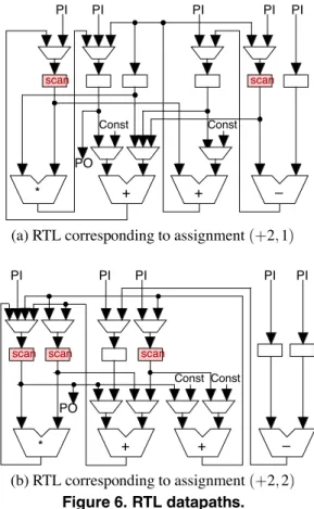
Example 3: Figs. 5 (a) and (b) show the pro- visional compatibility graph GC(G′sD1,+2,1) and GC(G′sD1,+2,2) for assignments (+2,1) and (+2,2) in G′sD1, respectively. The wights wp(+2,1) and wp(+2,2) are 40 and 220, respectively. Similarly, the others wp(+3,1) and wp(+3,2) are 230 and 40, re- spectively. Assignments(+2,1) and (+3,2) are min- imum, and hence assignment(+2,1) is selected here. Then, operation+2 is scheduled at step 1 by force- directed scheduling. Note that assignment(+3,2) re- sults in the same scheduling as(+2,1). After updat- ing mobilities and forces, the remaining unscheduled operation is+3 only, and accordingly +3 is assigned to step 2 with minimum force. As a result, a (com- pletely) scheduled DFG GsD1 is obtained. By apply- ing the binding algorithm [12] to GsD1, we can ob- tain an RTL datapath shown in Fig. 6(a), which re- quires two scan registers for acyclic structure. Fig. 6(b) shows an RTL datapath obtained by assignment (+2,2) instead of (+2,1) mentioned above and apply- ing the same binding algorithm. The RTL datapath cor- responding to(+2,2) requires three scan registers for acyclic structure. Thus, we can reduce the number of scan registers for acyclic structure by scheduling with
provisional binding. ✷
3.3 Experimental results
A force-directed scheduling algorithm in which our provisional binding is embedded was applied to exam- ples of data flow graphs (DFGs) GD1 and GD2. The
former GD1 is used in the above discussions. Table 1 shows the characteristics of DFGs. Columns #ops,
* + +
PO
Const PI
–
scan
Const scan
PI PI PI PI
(a) RTL corresponding to assignment(+2,1)
* + +
PO
Const PI
–
scan scan
PI PI PI
Const scan
PI
(b) RTL corresponding to assignment(+2,2) Figure 6. RTL datapaths.
#PIs, #POs and #vars denote the numbers of opera- tions, primary inputs, primary outputs and variables, respectively.
In order to analyze the effect of our method, we used two algorithms for scheduling and binding sev- erally, and tried all the combinations: (SS) force- directed scheduling algorithm with provisional bind- ing, (S) force-directed scheduling algorithm without provisional binding, (SB) binding algorithm by mini- mum weighted clique partitioning [12], and (B) bind- ing algorithm by minimum unweighted clique parti- tioning. In the same way as the above discussion, in the schedulings (SS) and (S), only the basic core of un- derlying force-directed scheduling algorithm is used, i.e., force represents the factor concerned with only the number of operational units. The latency constraints for GD1and GD2are both 5.
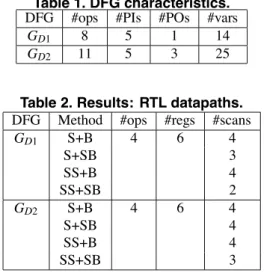
Table 2 shows the resulting RTL datapaths obtained by the combinations of scheduling and binding algo- rithms. Columns #ops, #regs and #scans denote the numbers of operational units and registers and the min- imum number of scan registers that are required for acyclic structure, i.e., for breaking all feedback loops, respectively. The numbers of operational units and registers are minimum under the latency constraint.
Table 1. DFG characteristics. DFG #ops #PIs #POs #vars
GD1 8 5 1 14
GD2 11 5 3 25
Table 2. Results: RTL datapaths. DFG Method #ops #regs #scans
GD1 S+B 4 6 4
S+SB 3
SS+B 4
SS+SB 2
GD2 S+B 4 6 4
S+SB 4
SS+B 4
SS+SB 3
From this table we can see that, by comparing SS+SB to S+SB (which corresponds to [12]), our schedul- ing method with the provisional binding reduces the number of scan registers. Furthermore, the number of scan registers by SS+SB is the smallest of all the algo- rithms, and the number of scan registers by SS+B is not smaller than that by S+SB for both examples, i.e., our scheduling method without the binding algorithm [12] for acyclic partial scan is not effective. This is because our scheduling with provisional binding performs on the premise that the following binding algorithm aims to the reduction in scan registers. Thus, the combina- tion of SS+SB results in the most effective in reducing scan registers for acyclic structure.
4 Conclusions
In this paper, we presented a scheduling algorithm for reducing the number of scan registers for acyclic structure. In order to estimate the number of scan registers during scheduling, we proposed provisional bindingof operational units. Results show that a force- directed scheduling algorithm in which our provisional binding is embedded can reduce the number of acyclic scan registers while keeping the area/performance op- timality.
We are now implementing the scheduling algorithm with the provisional binding. We shall show some experimental results for large benchmark data flow graphs at the Workshop.
Acknowledgements
Authors would like to thank Drs. Yoshinori Mat- suura and Hideyuki Ichihara of Hiroshima City Uni- versity for their helpful disscussions. This work was supported in part by Hiroshima City University under the HCU Grant for Special Academic Research (Gen- eral Studies) and by Foundation of Nara Institute of
Science and Technology under the Grant for Activity of Education and Research.
References
[1] T. Inoue, D. K. Das, C. Sano, T. Mihara, and H. Fu- jiwara, “Test generation for acylcic sequential circuits with hold registers,” IEEE/ACM Proc. Int’l Conf. on Computer Aided Design, 2000, pp.550-556.
[2] R. Gupta, R. Gupta and M. A. Breuer, “The BALLAST methodology for structured partial scan design,” IEEE Trans. on Comput., Vol.39, No.4, pp.538-544, April 1990.
[3] R. Gupta and M. A. Breuer, “Partial scan design of register-transfer level circuits,” Journal of Electronic Testing: Theory and Applications, Vol.7, pp.25-46, 1995.
[4] T. Inoue, T. Hosokawa, T. Mihara, and H. Fujiwara,
“An optimal time expansion model based on combina- tional test generation for RT level circuits,” Proc. IEEE Asian Test Symp., 1998, pp.190-197.
[5] S. T. Chakradhar, A. Balakrishman, and V. D. Agrawal,
“An exact algorithm for selecting partial scan design,” Proc. Design Automation Conf., 1994, pp.81-86. [6] M. Inoue and H. Fujiwara, “An approach to test synthe-
sis from higher level,” Integration, the VLSI journal 26, pp.101-116, 1998.
[7] T. C. Lee, N. K. Jha, and W. H. Wolf, “Behavioral syn- thesis of highly testable data paths under the non-scan and partial scan environments,” Proc. Design Automa- tion Conf., pp.292-297, 1993.
[8] M. Potkonjak, S. Dey, and R. K. Roy, “Behavioral syn- thesis of area-efficient testable designs using interac- tion between hardware sharing and partial scan,” IEEE Trans. on Computer-Aided Design of Integrated Cir- cuits and Systems, Vol. 14, No. 9, pp.1141-1154, 1995. [9] A. Mujumdar, R. Jain, and K. Saluja, “Behavioral syn- thesis of testable designs,” Proc. IEEE Int’l. Symp. on Fault-Tolerant Computing, pp. 436-445, 1994. [10] V. Fernandez and P. Sanchez, “Partial scan high-level
synthesis,” Proc. European Design and Test Conf., pp.481-485, 1996.
[11] M. L. Flottes, R. Pires, B. Rouzeyre and L. Volpe,
“Low cost partial scan design: a high level synthesis approach,” IEEE Proc. VLSI Test Symp., pp.332-340, 1998.
[12] T. Takasaki, T. Inoue, and H. Fujiwara, “A high-level synthesis approach to partial scan design based on acyclic structure,” IEEE Proc. Asian Test Symp., 1999, pp.309-314.
[13] P. G. Paulin and J. P. Knight, “Force-directed schedul- ing for the behavioral synthesis of ASIC’s,” IEEE Trans. on Computer-Aided Design, Vol.8, No.6, pp.661-679, June 1989.
[14] G. De Micheli, Synthesis and optimization of digital circuits, McGraw-Hill, 1994.