Beam beam Hirata 1992

Reprints available directly from the publisher

Photocopying permitted by license only Printed in the United States of America.

A SYMPLECTIC BEAM-BEAM INTERACTION WITH

ENERGY CHANGE

KOHlI HIRATA1, HERBERT MOSHAMMER2 and FRANCESCO RUGGIER03

1KEK, National Laboratory for High Energy Physics, Tsukuba, Ibaraki305,Japan 2SLAC, Stanford Linear Accelerator Center, Stanford University,

Stanford, CA94309, USA

3CERN, European Laboratory for Particle Physics, CH1211 Geneva 23, Switzerland

(Received8September1992;in final form8October 1992)

A mapping, called synchro-beam mapping, is proposed which describes the effects of the beam-beam interaction in presence of synchrotron motion. The mapping is symplectic in six dimensional phase space. In addition to the usual transverse kick, this mapping includes the bunch-length effect on the collision point and the energy variation caused by the electric field of the opposite bunch. The case of weak-strong interaction is investigated by simulation, showing that the beam-beam energy exchange has an influence on the distribution tail.

KEY WORDS: Beam-beam interaction, Symplectic map

INTRODUCTION

The perfonnance of many colliding storage rings is limited by the beam-beam interaction1.

A particle feels a nonlinear force produced by the encountering bunch at the collision. This beam-beam force acts mainly in the transverse directions so that the longitudinal effects have scarcely been studied2, except for the cases of a collision with a crossing angle3• Recently, however, high luminosity machines are being considered4,5,6 where the beams are focused extensively at the interaction point (IP) so that the beam sizes can vary significantly within the bunch length. Krishnagopal and Siemann⁷have shown that we should not neglect the bunch length effect in this case. The transverse kick depends on the longitudinal position as well as on the transverse position. If we include this effect, however, from the action-reaction principle, we should expect, at the same time, an energy change which depends on the transverse coordinates. Such an effect is reasonably understood from the fact that the beam-beam force is partly due to the electric field, which can change the energy8,9.

The action-reaction principle comes from the symplecticity of the reaction: the electro- magnetic influence on a particle is described by a Hamiltonian. The symplecticity is one

205

of the most fundamental requirements when studying the beam dynamics. A nonsym- plectic approximation can easily lead to unphysical results, in particular in proton rings. Also we will show some noticiable effects in e+e- case.

In this paper, we propose a simple, approximate but symplectic mapping for the beam- beam interaction which includes the energy change as well as the bunch-length effect. Some preliminary discussion is given in Refs.IO,II. In the next section, we propose the mapping in a Hamiltonian form, which directly assures its symplecticity. Then in Sect.3, we will study the nature of the mapping by interpreting its consequences. The mapping itself is quite general and can be applied to any distribution function. We show in Sect.4 how it appears when the distribution function is a Gaussian in transverse directions. The mapping is applied to the weak-strong case and some numerical results will be shown in Sect.5. The last section, Sect.6 will be devoted to discussions.

2 THE SYNCHRO-BEAM MAPPING 2.1 Accelerator Coordinates

The motion of a particle is described by the accelerator coordinates

(1) as functions of the distance s from the IP.

In a drift space, i.e. in the absence of any electric or magnetic field, x is related to the local Cartesian coordinates as follows: x and yare two transverse coordinates perpendicular to the direction of s, (Px,py) are the corresponding relativistic momenta normalized, i.e.

ｭｾ dx dy

(Px,Py)

=

IPol(dt' dt)' (2)

where

IPol

is the absolute value of the three-momentum p for the reference particle and

ｾ is the associated relativistic Lorentz factor. (We do not use the so-called canonical momenta, which include the vector potentials). We use

z == s - ct(s), (3)

(4) where c is the light velocity, t is the difference in the arrival time at s between the considered particle and the reference particle, (z (s)

>

0 means that the particle arrives at s earlier than the reference particle) and

Ipl-IPol

E -Eo

E - - - - -

- IPol -

Eo .

Here, the ultrarelativistic approximation is used so thatE ==c

_Ipi

holds.

We study the change ofx, Eq.(l), by the beam-beam interaction. Since both bunches move in opposite directions, we should introduce two kinds of s, s± for e± bunches. Of course

(5) Correspondingly,z+ andz_ have opposite directions.

2.2 Reduction of the Strong-Strong Problem to the Weak-Strong Problem

Since we are interested in the strong-strong case, we start with the 6-dimensional distribu- tion functions 7/J±(x;s) fore± bunches normalized to unity. We first make longitudinal slices of both bunches. Let us define the longitudinal distribution function A±(Z) as

(6)

Each value ofZ has its transverse plus energy distribution if±(x, y ,Px, Py,E;Z±, s):

(7)

This defines the distribution function of each longitudinal slice. It seems useful here to note that7/J(x;s) is not a distribution at a given time (snapshot image) but rather at a given position s, (streak image). Thus, the distribution of each slice, if(x,y ,Px, Py,E;Z±, s ==0), is evaluated when it passesｴｾ･ IP. At the IP (s± ==0), each slice may have^Z(O)±. Slices having the largest^Z(O)± first collide with each other.

Imagine that we have

7/J±

(s

±

==0), which carne out of the arc, without being affected by the beam-beam interaction. Actually, some particles should have been affected already. Thus this

7/J

is an ideal one. The slices havingz+(O)and z_ (0) collide with each other at (8)

A consequence is that the point where a test particle collides with the slice is not the IP(s ==0). We call this point the collision point (CP). It changes from tum to tum.

To apply the beam-beam interaction, it is convenient to introduce a virtual (or logical) time T. AtT, slices with Z+ andZ _ such that

(9) collide with each other. This T can vary from -00 to +00. An event occurring later (with respect to the virtual time) is influenced by the earlier events, but not vice versa. At eachT, we can consider the collision of a pair of slices, ignoring other pairs. Thus the study can be reduced to that of a collision between two slices.

The transverse beam sizes of the slices are kept constant during this collision, because the slice-slice collision takes place in an infinitesimally small time. Thus, when consider- ing the dynamics of ane+,for example, thee- slice is considered to be unaffected. The beam-beam force then can be treated as a prescribed force. For a single passage problem, thus, the problem is reduced to the so-called weak-strong case. Unless otherwise stated, we will study the effect of one slice (having z*) on a colliding particle. In this case, the slice is called the strong slice and the particle is called the test particle. Quantities concerning the strong slice will have a subscript

_*

and quantities without

_*

refer to the test particle.

2.3 The4 x 4 Treatment

Before going into detail, it seems convenient to recall the case where the synchrotron motion is negligible. In this case, the system is described by

(10) and the Hamiltonian for the beam-beam kick can be written as

(11) whereN* is the number of particles of the strong slice andQ

==

(Q1,Q2, ... )represents a set of parameters characterizing the transverse distribution function of the strong slice

'ljJ(x; s)== r¢(X4,s)8(s) : (12)

since the longitudinal extension is ignored, the whole bunch is represented by a single slice. It is well known that U is essentially the electric scalar potential of the strong slice:

U (x, y; Q(s)) ==- - 2ee*

_J

dT*In(IT - T*

I)

p(T*;Q(s), s), (13)

1fEe^Eo

whereE_eis the dielectric constant of the vacuum, ethe electric charge of the test particle, e* the same for the particles in the strong slice, T ==(x, y), and

(14)

This HamiltonianHbb induces a map

at the IP, where:A :denotes the Lie operator¹² defined by :A: x

==

[A,x].

(15)

(16) Here, [ , ] denotes the Poisson bracket. In this case, the normalized transverse momenta Px and Py change as follows:

(17)

(18) (i stands for eitherx ory). Transverse positionsx,y and longitudinal coordinates (z,E) do not change.

When r¢ is a Gaussian, only

(19)

are relevant parameters Q. In this case, we have

and

(20)

(21)

wherere is the classical electron radius. The explicit form of

fi,

for this case, is known as Bassetti-Erskine formula13:

Here w is the complex error function.

The map induced byH_{bb ,} Eq.(ll), is of course symplectic in 4 x 4 (even in 6 x 6) sense. If synchrotron motion is not negligible, however, we should proceed to 6 x 6 treatment.

2.4 The Synchro-BeamMapping

We propose a mapping for a particle-slice interaction, which is generated by

Here, n* is N*A*(Z*), the number of particles in the strong slice now considered, ,U is the same as Eq.(13) but the arguments are different:

y == y (y,py, z)==y +PyS (z, z*),

(24)

(25) with S standing for the location of the collision of the test particle(z) with the strong slice(z*) as seen from the test particle:

When1/J is a Gaussian, we have

(26)

Q*(s)==

(a;

(s),a;(s)) . (27)

Because of the presence of8(s), H_bb is applied to x at the IP. This gives a map from x/p to ｸＷｾｷＬ even if the collision takes place at the CP.

Let us perform the Lie operation.

(28) It is convenient to do it in a different canonical basis. Let us introduce a new set of canonical variables X

==

(X , Px , Y , Py , Z , Pz )^by

X

₌₌

x +PxS (z, z*), Px

==

Px, Y ==Y+PyS(z,z*), Py

₌₌

_Py,

Z P_z ^{P; +p}

2

==

z, _{］］ｅＭｾ}

They are related to the original variables x by

X

==

exp (: -D[S (z, z*)] :)x, where

p2 +p2 D[s]

==

^{_x_ _}y s.

2

In these new variables, the Lie transformation Eq. (28) can be written as X;;w

==

exp(: -n*U :)X/P ,

where

U ==

^e-:D:Ue+:D:

==

^U (X, Y,Q*(S (Z, z*))). Thus the map is a function only of coordinates.

We find that(X, Y ,Z) remain unchanged

(X,Y,Z)new

==

(X,Y,Z), but

(

px) (Px -fx(X,Y;Z) ) exp(:-n*U(X,Y;Z):) P y

==

Py-fy(X,Y;Z) ,

P_z P_z -g(X,Y;Z) where

(29)

(30)

(31)

(32)

(33)

(34)

(35)

fx(X, Y;Z) fy(X, Y;Z) g(X,Y;Z)

(36)

Note that the Z derivative in the last expression is applied through Q so that it should be written as

(37)

Going back to the original variables x, we get the explicit form of Eq. (28):

Xnew p;ew ynew p;ew znew

x+S(z, z*)!x(X, Y;Z), Px -!x(X,Y;Z), y +S(z ,z*)!y (X , Y; Z), py -!y(X,Y;Z), z,

E

_-1

fx (X, Y: Z)fpx

_-1

fx (X, Y: Z)] -2!Y(X,Y,Z)[Py - 2!Y(X,Y,Z)] - g(X,Y;Z).

(38)

The above map, from XIP to ｸＷｾｷＬ is called synchro-beam map, because it includes the coupling between transverse and longitudinal motions due to the beam-beam interaction. It is clear that the synchro-beam mapping is symplectic for any distribution ｾＪ of the strong bunch, since it can be derived from the general Hamiltonian Eq. (23).

Some points should be noted:

1. We could first derive the equations of motion and integrate them afterwards to obtain Hbb. Special care should be taken in integrating dpx / ds because it depends also on Px. This approach can be found in Ref.11 •

2. The synchro-beam mapping is applied at the IP (s

==

0), although the real collision takes place at s

==

S(z, z*), called the collision point (CP). This is a favourable point of our mapping: usually, tracking codes provide the development of x for the arc, which is from IP to IP. Thus, it is desirable to apply the beam-beam mapping at the IP.

3. The mapping, Eq. (30), is of course symplectic, but does not correspond to a real evolution of x in a drift space: because, in the drift space, the energy ^E could not change. It would be so if S(z, z*) did not contain any canonical variable. Since, however, it is closely related to the drift map, we call the mapping, Eq. (30), virtual drift mapping.

4. Relatedly, the variable X, Eq. (32),can be identified with the coordinate x at the CPo Since, in tum, the CP is a function ofz, one may be lead to a 'mysterious' expression z (s(z )). By relating it to XIP through the virtual drift, we can avoid this confusion. 5. The potential U, used in Hbb, Eq. (23) was related to the electric potential. In the

4 x 4 case, we can add any constant to it. In the synchro-beam mapping, it should be treated more stringently. Only U, defined by Eq. (13) should be employed. (An exception: addition of a constant to the particle-particle potential is acceptable: it does not lead to any additionalz-dependent term). For example, an alternative potential¹⁴ may be used in 4-dimensional treatment but should not be used in the synchro-beam mapping: the z-derivative diverges whenr ｾ ^00.

6. When considering -the slice-slice interaction, Eq. (36) insures the energy-momentum conservation of the two-slice system. It is partly due to the ultra-relativistic approxi- mation. There is no long-range longitudinal force.

7. We have neglected the effect of the solenoid field, which exists almost always because of the needs of high energy experiments. Itis, however, a different effect and should be studied separately.

8. By the synchro-beam mapping, thez does not change. This fact justifies our discussion relying on the concept of the slices. Mixture of particles between two slices does not occur during a single passage of the IP. This is due to an approximation of the drift space Hamiltonian which can be justified for usual ring parameters. See discussion given in section 6.1.

3 INTERPRETATION OF THE MAPPING

We have given the map, which is surely symplectic. How reasonable is it? We shall now discuss the physical meaning of our map.

3.1 Floating Collision Point

The calculation of the Lie operation, given in the previous section, shows that the whole mapping consists of three successive mappings:

(39) The equation appears to be applied at the IP (s==O), whereas the real action takes place at the CP (s

=

S(z ,z.». It seems convenient here to give a physical interpretation of the nature of the mapping.

The first step of Eq. (39) is the virtual drift mapping, Eq. (30) from the IP to CP, the second is the beam-beam mapping with respect to the variable X, Eq. (32), and the last step is the inverse of the virtual drift mapping. We can say that the whole mapping expresses the collision effect at the CP in terms of the canonical variables defined at the IP.

In this c6nnection, it is worth noting here how to handle the successive collisions with many slices. Imagine that there areL strong slices, each having

_nt

particles and each havingz.

=

z;*. Physically, the test particle first collides with the slice i=l, then with 2 ... L. (We assume

_zt > z2 ... zn.

The whole process can be written as

x7ft

^w

=

･ｸｰＨＭｮｾ :U(SI) :)exp(-n; :U(S2):)"·exp(-n{ :U(Sd

_:)x/p,

(40) where Si

₌

S(z ,

_zn.

Note the. order of the Lie operation: it is the opposite of the physical ordering*.

The effect of the drift from one slice to the next is already included in Eq. (40). With L slices for the strong bunch, we should only applyexp(

_{-nt :}

U (Si) :) for L times in the order of the virtual time T. The following formal expression is useful:

x7r

= Texp[-N.

_f:

dz.}..(z.,s = O)U(S(Z,z.»] X/P, (41)

* The reason is that the Lie operator operates on the function but not on the numbers.

where T denotes the time ordered product with respect toT(Z,z*). (From left to right for

T small to T large, with ^Z fixed.). When A*(Z*, 0)

==

8(z*), Eq. (41)reduces to Eq. (15).

3.2 The Electromagnetic Field due to a Bunch Slice

One of the consequences of the fact that the CP is different from the IP is that the electric field has a longitudinal component: even if the IP is a symmetry point, the CP is not.

In this subsection, we will give a physical interpretation of the synchro-beta mapping in terms of the electromagnetic field produced by the strong slice. Thus all quantities should have subscript*. For the sake of brevity, however,

in this subsection, the coordinates always follow the sign convention for the strong slices. It is not meant to give the 'exact' derivation of the electromagnetic field: here we should replace Px,y as

(px ,py) - - t (xI ,Y')

==

(dx / ds, dy/ ds). In this respect, refer to the discussion given in section 6.1.

Let

(42)

(Ex(X-XI,Y-YI),Ey(x-XI,Y-YI))

_=-2-1

^{e r - rl1}_{2 '} (43)

1fEe r - rl

be the transverse components of the electric field vector at r produced by an e+ at rl. Here, r

==

(x,y). Since in the extreme relativistic limit the electric field is perpendicular to the velocity of the source particle, VI ex (xL

yf,

^{1),we have}

E· VI

==

0 and hence

Thus the total integrated electric field produced by the strong slice has components EAr)

=

n

_J

dr]Ex(r - r])p(r]),

Ey(r)

=

n

_J

dr1Ey(r - r])p(rl), and

(44)

(45)

(46)

(47)

Ez(r) = -n

_J ､ｲ｝､ｱ｝､ｅＨｸｾｅｸＨｲＭｲ､ＫｹｾｅｹＨｲＭｲ｝ＩＩＧﾢＨｲｉＬｅＩＬ

⁽⁴⁸⁾

Hereqi

==

(x{,y{) and

p

is the distribution function in the coordinate space

p(x,y) =

_J

dqdE'¢(x,x',y,y',E), q = (x',y'). (49) The transverse components (Ex, Ey)are derivable from

U(r - rI)

==

- - I n (Ir - rII),e

21fE_e ⁽⁵⁰⁾

by

(51) If we define the total averaged electric potential

we have

(52)

(EAr),Ey(r») = -

_{ＨｾＬ ｾ}

) <!J(r;Q(s». (53)

Note that

E

and 0 have dimensions of electric field x length and electric potential x length, because they are produced by a slice.

Now, we relate0to

E

z ,Eq. (48). The distribution function of the strong slice

(J

obeys the equation corresponding to the drift space:

(54)

From Eq. (48), we have

Ez(r)

=

-n

_J

dr1dql

ＨｸｾﾣｸＨｲＭｲｬＩＫｹｾﾣｹＨｲＭｲｬﾻＩＧｉＬＳＨｲｊＬｅＩ

+n

_J

dr1dql

ＨｸｾＡｦＭＫｹｾｦｉＣＩＧｉＬＳＨｲｬＬｅＩ

-n

_J

dr1dql

_{Ｈｸｾｩｦ ＫｹｾｾＩ}

'I,3(rJ,E)

n

_{J ､ｲｬ､ｱｬＨｘｾｾ ＫｹｾｾＩｕ}

-n

_J

dr 1dql(as

'l,3)U

--9s<!J (55)

In summary, we have

(56)

3.3 Electromagnetic Field Feltbya Test Particle

We now return to the test particle and recall the convention of *. Since U is a scalar function, Eq. (56) holds also true in the coordinate frame of the test particle:

- - - 8 8 8

(Ex,Ey,Ez)==-(-a'-8 '-8 )0·

x y s+ ⁽⁵⁷⁾

Since theU in the definition ofH_{bb ,}Eq. (23), is the electric potential, it can be identified with <jJ, defined by Eq. (52):

e<jJ

- :=:n*U. (58)

Eo

from Eq. (13) and Eq. ＨｾＲＩＮ Both are the same thing except for a constant factor. From Eq. (36), using

a as a

az az as

we can then identify (fx ,fy ,g) as

1

_a

laS'

⁽⁵⁹⁾

Ix

fy g

e - -EoEx }

Ｍｾｅ evaluated at theCPo ｅｾ ｾ

-2EoE^z.

We thus can express the synchro-beam mapping, Eq. (38) as

(60)

(61) x new

y^new p;ew znew

E^new

+eS(z , z*) E CP

x E x '

e 1J_cp Px+ EoEx ,

+eS(z , z*) E CP

Y Ej) y '

e ECP py+ Eo y ,

z, e -CP e -CP

E +2EoEx [Px + 2Eo Ex ] e -CP e -CP +2EoEy [Py - 2Eo Ey ]_{e -CP} + 2EoEz .

The change of the transverse momenta is due to the transverse electric field. Actually, the magnetic field gives the same effect. Thus the transverse electric effect should be multiplied by 2 but it should be divided by 2 again due to the fact that the test particle crosses the strong slice in half the time it would take if the slice did not move and sit at theCPo The latter effect will be refereed to as the 'time-of-flight' effect. The change of transverse coordinates is due to the floatingCP. The change ofEis more understandable in the form

DE

ｾ

_Eo ^{(lE Cp}₂

ｘｾｬ､

⁺

ｸｾ･ｷ

^+lEcP

ｙｾｬ､

⁺

ｙｾ･ｷ

^+lECp)

x 2 2 y 2 2 z

ｾ _{(lECpx '}⁺lECPy'+lE Cp )

Eo 2 x 2 y 2 z

Because of the electric field, the test particle can change its energy as

(62)

dE e ce ^{I ,} (63)

-d :=: -E·v:=: -(Exx +EyY +Ez).

t Eo Eo

The magnetic field does not contribute to this effect. Because of the time-of-flight effect, we have an extra factor (1/2) in Eq. (62). To the best of our knowledge, this effect was

first realized by Bassetti^8, although the possible presence ofEz was not considered at that time. Augustin²pointed out the possibility of energy change due to the beam-beam force. His argument, however, was not clear enough. He asserted that, in the rest frame of the strong slice, the change of momentum of the test particle is always perpendicular to its momentum. We should say, instead, the change is always parallel to the electric field.

We have presented the synchro-beam mapping, which is symplectic, and have shown that it allows a reasonable physical interpretation within an approximation that (Px,py)ｾ

(x',y'). (See discussion given in section 6.1.)

4 GAUSSIAN DISTRIBUTION

The discussion thus far is quite general: it applies to an arbitrary distributions of the strong slice. It is useful, however, to see how the synchro-beam mapping looks like for simple but realistic distributions. Here we consider the round Gaussian and bi-Gaussian distributions. In the following calculation, there is no need to specify the longitudinal distribution A*(Z*).^I This becomes necessary only when we calculate the successive application of the synchro-beam mapping as in Eq. (41).

4.1 Round Gaussian Distribution

The round-Gaussian distribution provides us the simplest non-trivial example, although this might me still too simple as a realistic model. We will use it for the illustration of the mapping and later for the weak-strong simulation. The distribution function is parametrized as

'"' 1 [ 1 -1

_t]

'!f;(r,p"s) = 27fy'detL:(s) exp -2(r,Pr)L:(s) (r,Pr) , where ｾ is a2x2 matrix

(64)

(65) In this model, we assume a perfect symmetry with respect to the rotation in the x-y plane and consider only one radial direction

_r

_ｾ

_Jx

²+y2. We also omitted the c dependence ofi/J because it is irrelevant in calculating the beam-beam force.

Since, in a drift space,

(66) we have

Ell(s) E_12(S) E_{22 (S)}

Ell (0)+2E 12(0)S+E 22(0)s2, E 12(0)+E 22(0)S,

E 22(0).

(67)

Thus the envelope ofi/J(s) is uniquely determined by that ofi/J(O). These formulae can be used to evaluate the beam-beam force at the CPo

The potential U is given by

The radial kick at the CPis

( .f +:) _ (x,Y).F

vX ,JY - Jr,

r It can be written as

(69)

(71)

2n*r

^{e .[}

-r

² ] (70)

fr

== - - -

exp( ) - 1. -

ｾｯｲ ＲｾＱＱＨｓ (z, z*» On the other hand, according to Eqs(36) and (37), we have

1 dII

_a.

1 d^ll Nr

e[. (

-r²). ]

g =

_ｮＪＲｾ

oE_llU = n*E_ll

_ｾ

2')'0 exp 2E_ll ^.··

In Eqs. (70) and (71), we use Eq. (67) to evaluate ｾｬｬ (S(z, z*».

We substitute (Ix,fY,g) thus obtained into Eq. (38) to obtain the synchro-beam map- ping in the present case:

where

r^new

ｰｾ･ｷ

znew

r +S(z , z* )fr , Pr - fr, z,

E -

1!r(Pr - 11r) -

g,

(72)

!r =

2n*r

^e _{1[.1_}

exp (. (r₊

_S

(z, Z*)Pr

_{)2). ]}

(73) 1'0 r + S (Z ,Z*)Pr ＲｾＱｬＨｓ (Z ,Z*» . '

ｧ］］｛｟ｉ｟Ｎｾ｝ ^xn*reexp(

(r+S(z,z*)pr)2). (74)

. _ｾｬｬ ds s=S(z ,z*) _ＲｾＰ . _ＲｾＱＱ (8(z,z*»

When studying the weak-strong effect, where one of the beams is considered to consist of only one particle so that the other beam can be assumed to be unaffected, we can use

( {3(s)

ｾＨｳＩ

==

Eo·· -a(s) ^{-.a(s) )}_{ｾＨｳＩ .} ⁽⁷⁵⁾

Here,EOis the nominal emittance and(n,ｻＳＬｾＩ are the Twiss functions. On the contrary, in the more realistic strong-strong case, the beam envelope E is perturbed by the beam- beam force, partly through the dynamic beta^l5and the dynamic emittance^l6effects. As long as the IP and its surrounding can be assumed to be a free drift space, Eq. (67) holds in any case.

We have derived the synchro-beam mapping using direct differentiation ofU. Note that there is an alternative way to obtain(Ix ,fy ,g) based on a calculation of the electric field10. Although, of course, the resulting mapping is the same, the calculation shows us that our interpretation of the mapping was right.

4.2 The Bi-Gaussian Distribution

Inthe bi-Gaussian case, the direct evaluation of the longitudinal field seems quite com- plicated. We derive the term g by a direct differentiation of U, according to Eq. (37). The transverse forcesfx andfy are already known: they are given by Eq. (22)with a's evaluated at the CPo

Without loss of generality we can assume that ax

>

ay. According to Eq. (37), the total effect of the longitudinal electric field is described by

n*

_(d

^x aU dyaU ) g(x,Y,_{ｾｸＬ ｾｹＩ} =

₂

ds_｡ｾｸ +ds_｡ｾｹ . We thus have to evaluate

(76)

and _｡ｾ

^a

ｕＨｸＬｙＬｾｸＬｾｹＩＮ y

(77)

Here, we have introduced an abbreviation ｾｾｩｙ ⁼ ｾｸＬｹＮ Using the following substitutions

2 Ｒｾｹ +u

t - ^{ｾＧＭＭﾭ}

- _Ｒｾｸ +u'

r= - ,ax

a y ⁽⁷⁸⁾

the beam-beam potential Eq. (21) becomes r

_II

U(a,b,r) = _Ｒｾ

1'0 r

ea2(/2-1)+b2(1-1/12)

- - - : : - - - - d t

(t2 - 1) ⁽⁷⁹⁾

and the derivatives of the potential can be written t as

a

Ｒｾ

｡ｾｹ ｕＨｸＬｙＬｾｸＬｾｹＩ

=

ｉＧｯＨｾｸ ^_ ｾｹＯｹＨ｡Ｌ｢ＬｲＩＬ where the integralsIx and I_y are given by

(80)

(81)

t These derivatives should be computed using the original form of the potential U(x,y,I:_{x ,}I:y ),Eq.(21), and then performing the change of variables. Otherwise, in differentiating Eq. (79) directly, one should be careful to take the limit fort -+ I in the upper extreme of the integral (corresponding tou -+ 00): this can be done only after the derivatives have been computed.

Integrals Ix and I_yare proportional to the second order derivatives of U(a,b,r) with respect to a or tob. Indeed from Eq. (79), we have

Recalling that

1 8²U

ＴＨｾｸ - ｾｹＩ ^{8a2 '}

1 8²U

ＴＨｾｸ - ｾｹＩ 8b^{2 . (84)}

fy +ifx

_ｾ

n* (88 + i_y

_{a 8)}

U

= J

^n*

₍₈₈

_b ^{+ i 88 ) U, (85)}

x . ＲＨｾｸ - ｾｹＩ a

and using Eq. (22), we finally obtain

(86)

(87)

Note that these two expressions tend to 0 when (x, y)---7 00.

Replacing ＨｸＬｙＬｾｸＬｾｹＩ in Eq. (76) and above expressions by ＨｘＬｙＬｾｸＨｓＩＬｾｹＨｓＩＩＬ

we obtain the necessary expression.

5 WEAK-STRONG SIMULATION FOR ROUND GAUSSIAN BEAM

In this section, we will investigate the numerical consequences of the synchro-beam mapping. Although it is not meant to give fairly realistic and practical predictions, it would be interesting to see some numerical results. Here we restrict ourselves to the simplest case: we study the round Gaussian beam and assume the weak-strong situation. The code includes betatron and synchrotron oscillations with damping and noise, associated with synchrotron radiation in the arcs of an e+e - storage ring. It also contains the bunch length effect of the strong bunch.

5.1 The Program

The program tracks each particle as follows:

5.1.1 Synchro-Beam Interaction For the sake of brevity, we rescale the canonical vari- ables as follows:

(88)

where ｏＢｾＬ ｏＢｾ and ｏＢｾ are the nominal values at IP of the transverse beam size, bunch length and relative energy spread, respectively. Note that the transformation to these variables is not symplectic. In terms of these variables, the synchro-beam mapping for a collision between a particle in the weak beam and a strong slice having z* is expressed as

Q^---+ Q-R1(Z -Z*)8P, P ---+P+8P,

Z---+Z,

£ ^---7£+R28P(P +8P/2) -G, where

(89)

(90)

(91)

(92)

ｏＢｾ co

R¹== 2r-l ' R²== - 2Or-l ' jJ/P 0"EjJ/P

Here, 17 is the nominal beam-beam parameter:

(93)

N*re (94)

17= = - -

41r'"'(co'

where co is the transverse nominal emittance of the strong beam. The denominator of Acol represents the variation of the beam size (of the strong slice) due to the floating effect of the CP" See Eq. (67).

5.1.2 Bunch Length Effect The necessity of introducing multiple slices was stressed by Krishnagopal and Siemann⁷.

In the multiparticle tracking, the longitudinal distribution function in Eq. (6) can be replaced by

L

A*(Z)==LWi8(Z - zt), LWi== 1.

i+l

(95) We considerL longitudinal slices. Let us make these slices in such a way that each slice has the same number of particles(Wi=const) and let us represent each slice by its longitudinal barycentre. The i-th slice then sits at

zt =

_ｾ

(exp(-(zti+I)2/2) - exp(-(zt_li)2

/2)) ,

y 2 1 r ' , ⁽⁹⁶⁾

whereｺｩｾｩＫｬ is the border between i-th and (i+l)-th slices. For example, whenL== 5, we have

zt(barycentre) :-1.3998, -0.5319, 0, 0.5319, 1.3998,

ｚｩｾｩＫｬ ^{(border) : -0.84159,} -0.2533, 0.2533, 0.84159. Each barycentre represents 1/5 of the whole particles.

5.1.3 Oscillation The transformations from IP to IP are just rotations with damping and quantum diffusion.

Thus we first apply the mapping

(

_ｾ

) - + U (21fvx ) (

_ｾ

) , (

_ｾ

) - + U (-21fvs ) (

_ｾ

) ,

(97)

(98) where

U(n) == (

_｣ｯｾｮ

-SInn

sinn) .

cosn ⁽⁹⁹⁾

5.1.4 Radiation For transverse diffusion, the symmetric prescription16is used, which is suitable for the case where the integer part of the betatron tune is much larger than unity. The longitudinal diffusion should be applied only to£,becauseV_sis usually much smaller than unity. Thus,

(100)

p - +

>'x

^P +

_{VI -} >';"2,

⁽¹⁰¹⁾

E

- +

>.;E

+

_{VI -} >':"3,

⁽¹⁰²⁾

where the P's are independent, random Gaussian variables with unit standard deviation. Here the A'Sare damping factors defined by

(103) where the T's denote damping times normalized by the revolution time, or equivalently the number of beam-beam collisions per betatron and synchrotron damping times, re- spectively.

5.1.5 Independent Parameters In the synchro-beam mapping, we introduced many variables. The essential parameters, however, are not so many. In the round-Gaussian case, the only dimensionless free parameters are the following:

• Nominal beam-beam parameter1],which is proportional to the total number of particles in the strong bunch.

• Transverse and synchrotron tunes V_x andvs ,

• Transverse and synchrotron damping timesTx and TE ,

• Ratios R1 and R2 •

10

8

6

4

2

o o ^0.05 0.1 0.15

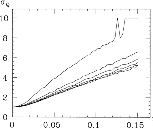
FIGURE 1: Transverse beam sizeaQ as a function ofTfwith different numbers of slices, L: those with L= 1 to 6 lie from top to bottom. Parameters: V_x= 0.15,Us ₌₌0.085, TE==200 andT_{x ==}400, R1==10, R2==0.

The ratioR1 represents a geometrical effect of the floating collision point: beams have different sizes at different CP's. The ratioR₂ represents the energy kick associated with the transverse kick. For usual parameters ofe+e - colliding rings, R2 is very small: this is at most 10-²,representing the fact that the longitudinal emittance is much larger than the transverse emittance.

5.2 Results of Simulation

5.2.1 Dependence on the number of slices In Fig. 1, the rms transverse beam sizes (104) are shown as a function ofTJ with changing L. Since R1

₌₌

lOis large, the effects of the floating collision points are a little ･ｸ｡ｧｧ･ｲ｡ｴ･､ｾ

For small values ofL, the results depend on it significantly, being consistent with Ref.? We may conclude thatL

==

5 is sufficient.

'"./

6

4

2

II II II II II

, _.

/

.

,.

\ /

.

_,

i II ,..

.'

^{\ . '}

_,

. ,'. I ' /

II \. I· .

,

f./ I·

·1 I·

·1 II I·

.,

II

,.

·1 _/1 I·

1 ^{. I}

l.

^,

,

'1

^.

. I I . I

/

_i.'

o o 0.1 0.2 0.3 0.4 0.5

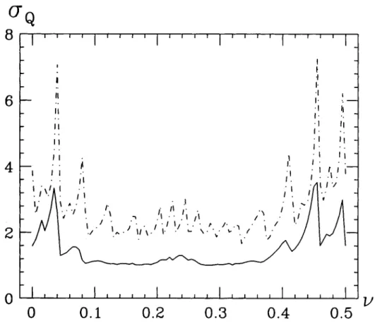
FIGURE 2: Beam size^I7Q as a function of^Vx with different value of slices,L: L = I (dotted line) and 5 (solid line). Parameters: Vs = 0.085,T.= 200 andTx= 400,1]= 0.05,R1⁼ 1,Rz = O.

5.2.2 Tune Dependence In Fig. 2, equilibrium transverse beam size is shown as a function ofV_{x '} The synchro-betatron resonances near

2v_x ± ^Vs ｾ ^{integers, (l05)}

are the most dangerous. This comes from the bunch-length effects represented by RI •

The energy kick effect, represented by R2 does not change the situation, except for the case of unrealistically large value of R_z. For comparison, we have shown the case with L

₌

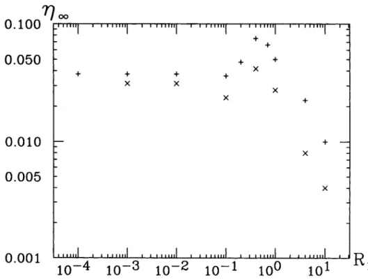
1 too. The reduction of the simulation results by the floating CP effect seems almost universal for various values ofV_{x '}

5.2.3 Beam Blowup When the current, i.e. the "7, increases, the beam sizes increase too. To parametrize this effect, let us define "700 by the value of"7 where(JQ

₌

2. The corresponding real beam-beam parameter, ｾｯｯＬ is four times as small as "700' because we use the real beam size in the latter case. (Note that the "7 is proportional to the current, whereas theｾ is proportional to the luminosity, apart from the possible "hourglass effect"17, 18. In Fig. ＳＬｾＰＰ is shown as a function of R_I for two very different values of the damping time.

O. 100

7]rr oo

TnlTT---,-TTTl"TT1r-...TTTT1,-r--,orrTnlTT---,-TTTl"TT1r-..."TTTT1rn-..-.

0.050

0.010

0.005

+

+ +

+ ⁺

+ + ₊ ^X

X X

X

X ₊

X

+

X

0.001

FIGURE 3: The maximum value of the nominal beam-beam parameter1)as a function of R ,. The parameters are l/x

₌

0.15, l/s

₌

0.085, (Tx ,Td

=

(4000,2000) (x) and (2000,200)(+)and L

=

5. The 'maximum' is defined such that a becomes twice as large as ao.

In this connection, it is interesting to note that, in Fig. 3,

(106) holds for R1;SI and when Tx and T, are fixed. This is consistent with a phenomenological observation^l9that the limiting value of the disruption parameter,Doo , is almost universal. Here

(Js

D oo

=

ＴＷｲｾｯｯ f32

=

ＸＷｲｾｯｯｒｉＧ (107)

Another interesting observation is thatｾｯｯ seems to have its maximum (perhaps a local maximum) at around R₁

=

1/2,which corresponds to f3x

=

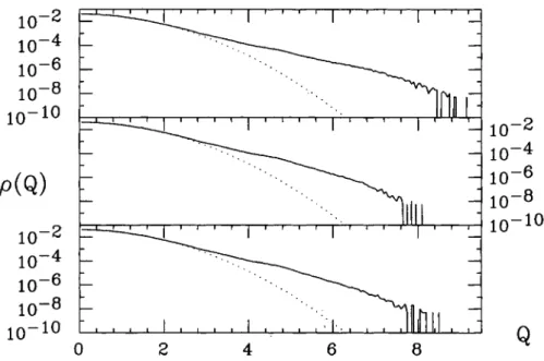
ＨｊｾＮ This fact seems to be consistent with the observation at CESR2o.

5.2.4 Tail Distribution The multiparticle tracking results given thus far may appear to imply that R₂ is not an important factor and can be ignored at least for electron rings. Actually, however, the energy change may influence the long tenn behaviour of the particles. In particular, the tail distribution may be modified.

In Fig. 4, we show the transverse distribution p(Q)+p(-Q) for different values of R2. Even when R2

⁼

0, the transverse distribution deviates from a Gaussian in the

Q

10-2 10-⁴ 10-6 10- 8

,J-,----r--lr-l _{10 - 10}

8 6

4

o

2 10- 2 10-4 10-6 10-⁸ 10- 10

10- 2 10-⁴ 10-

⁶

10-⁸ 10- 10

p(Q)

FIGURE 4: Transverse distribution for three values ofR2: R2

₌

0 (bottom),R2

₌

0.01 (middle) andR2

₌

0.1 (top). The horizontal axis isQ, the normalized distance from the origin, and the vertical the distribution in Q. The data was taken for 100 particles and through 2 x 10⁶turns. Parameters: Vx = 0.15, Vs = 0.085, T.

₌

200 andT_x

₌

400, 11

=

0.1,RI

₌

0.5 andL

₌

3. Dotted lines correspond to the case 11

=

O.

4 6 2

10-² 10-

⁴

10- 6 10-⁸ Ｏ］｣ＺＺＺＺＺＡ］ＺＺＺＺＺＡ］］］ＭＭＮＭｲＭＭＮＭ［ＭＭＭＭＮＭＭｲｾｾＭｲＭＭＫＭ｟ｲ｟Ｇｩ ^{10 - 10}

o

10- 2 10- 4 10- 6 10- 8 10- 10

10- 2 10-⁴ 10- 6 10- 8 10- 10

FIGURE 5: Energy distribution for three values ofR2: R2

₌

0 (bottom),R2

₌

0.01 (middle) andR2

₌

0.1 (top). The horizontal axis isEand the vertical the distribution inE. The data was taken for 100 particles and through 2 x 10⁶turns. Parameters are the same as Fig. 4. Dotted lines correspond to the case 11 = O.

tail. This is a well-known effect. We superposed the nominal (TJ

==

0) distribution for comparison by dotted lines. The tail does not contribute to the rms beam sizes so that the nominal Gaussian fits the central region very well. The non-Gaussian tail in the transverse direction does not affect the luminosity, as long as the central part is not seriously modified. This, however, may influence the background to the detectors as well as the lifetime.

The effect of R2 is remarkable in the further tail. It appears that the further tail for R2

⁼⁼

0.01 is smaller than that for_R2

==

0: for_R2

==

0.1 it is larger.

We show similar graph for the energy distribution in Fig. 5. In this case, bothR1and R2are important parameters. ForR2

==

0 (the bottom) the distribution should be exactly the nominal Gaussian: the tail part deviates from it only because of the finite number of data. Within this uncertainty, however, theR2 has a certain effect on the tail. This tail is the direct consequence of the synchro-beam mapping.

6 DISCUSSIONS 6.1 Chromatic Effects

In interpreting the synchro-beam mapping, we have regarded

Actually, there is a difference: dx ds

Px rv - .dx ds

---;:========================Px

_#

Px .

( ^{M)2 _p2_p2}

_IPol

x

_y

(108)

(109)

(110) The8x',should depend on the energy, ^E. This energy dependence of the transverse kick is one of the sources of chromaticity.

We have used the above approximation only in the virtual drift map: we should have used

x(s)

==

x(O)+ Px s.

ｊＨｅＫｾｏＩＲ｟ｰｊＭｰ［

This will make a difference in 8x between particles having the samePi'S but different

E'S. This makes also a tiny change ofz (path length effect) during the whole beam-beam collision and thus brings a difficulty in using the concept of the longitudinal slice. What we have neglected is just this chromatic effect over the bunch length. This is, however, quite small when compared to the chromatic effect over the whole drift space. We can ignore it for the usual parameters ofe+e- rings.

Our mapping, or the Hamiltonian, Eq. (23), does not depend on E. This should be so for the same reason that the Hamiltonian of a thin quadrupole magnet does not depend on E. We have assumed that there is no longitudinal magnetic field. With electric field

and transverse magnetic field, the Lorentz equation says that the changes of Px, Py and

Ipl

do not depend on energy.

In the present scheme, thus, the chromatic aberration of the beam-beam force, if any, will appear only through the arc.

6.2 Importance of the Synchro-Beam Mapping

The synchro-beam mapping proposed in this paper is important for two reasons. First, it provides us a 6 x 6 symplectic map. This enables us to install the beam-beam interaction in 6-dimensional tracking code. If the bunch-length effect is ignored, we can do it by using the 4 x 4 version. But if we want to include the bunch length effect, the only possible way is to use 6 x 6 formalism. The widely used technique of using 4 x 5 mapping, which includes the bunch-length effect on the transverse motion but does not include the energy-change depending on the transverse coordinates, explicitly breaks the symplecticity. Absolutely, this cannot be used for proton machines.

Relatedly, one may ask 'can we ignore R₂ in Eq. (89) for e+e- colliding rings?' The answer is 'yes', if we are interested only in the equilibrium rms beam sizes. The answer would be also 'yes', if we could stand the breaking of symplecticity. If we put R2 ^---+ 0 in a coordinate frame used in the multiparticle tracking, Eq. (88), we cannot return to the original physical variable x: the limit corresponds to a singular point of the transformation. PuttingR2 ==0 while keepingR1

i=

0 corresponds to an unphysical situation that the energy spread is infinitely large but the bunch length is finite.

In presence of strong synchrotron radiation, one may say that the symplecticity is less important than for proton rings. For the rms beam sizes and the central distribution, it may be true, as shown by the simulation. But the statement still needs the proof. As we have shown in the simplified multiparticle tracking, in addition, for more delicate issues such as the tail distributions, however, the loss ofR_{2 ,} i.e. the loss of the symplecticity may cause a serious errors even in the electron case.

6.3 Conclusion

The synchro-beam mapping is a fairly accurate, though not 'exact', model of the beam- beam interaction. It is symplectic in 6-dimensional sense for an arbitrary distribution for the beams. It applies both to weak-strong and strong-strong cases. It has a reasonable physical interpretation. We of course do not reject less accurate treatments, such as 4 x 4 treatment or 4 x 5 treatment (longitudinal distribution can affect transverse dynamics, but not vice versa), as long as the synchro-beam effects seem ignorable. The claim on the luminosity is, however, increasing rapidly. Thus the beam-beam interaction should be studied more and more carefully. In this situation, we should use the most accurate method available to treat the beam-beam effects. Theｾｹｮ｣ｨｲｯＭ｢･｡ｭ mapping is a good candidate for this purpose. More detailed and extended works should be relegated to the future, including the strong-strong simulation (it requires a tremendous CPU time to do this job reliablly enough) and long-term single particle tracking with lattice nonlinearity.

ACKNOWLEDGEMENTS

This work started when K.H. and H.M. stayed at CERN. They thank members of the CERN SL-AP group for the hospitality extended to them. M. Bassetti is acknowledged for raising authors attention to the energy loss due to the electric field. They thank also M. A. Funnan and A. Piwinski for sending them valuable comments.

REFERENCES

1. The most recent overview of these issues can be found, for example, in the Proc. Third Advanced ICFA Beam Dynamics Workshop on Beam-Beam Effects in Circular Colliders 29 May, 1989, 1. Koop and G. Tumaikin, Editors, Institute of Nuclear Physics Publication (1990).

2. J. Augustin, Orsay, 36-69 (1969).

3. A. Piwinski, IEEE Trans Nucl.Sci. NS-24 1408 (1977).

4. Accelerator Design of the KEK B Factory,(Eds. S. Kurokawa, K. Satoh and E. Kikutani), KEK Report 90-24 (1991).

5. An Asymmetric B Factory - Conceptual Design Report,LBL PUB-5303, SLAC-372, CALT-68-1715, UCRL-ID-l 06426, UC-IIRPA-91-01 (1991).

6. Feasibility Study for a B Meson Factory in the CERN ISR Tunnel, Ed. T. Nakada, CERN 90-02 (1990). 7. S. Krishnagopal and R. Siemann, Phys. Rev. D41,2312 (1990).

8. M. Bassetti, Longitudinal Energy Changes in a Bunch, LNF-T-I05 (1978).

9. M. Bassetti, Come Migliorare gli Attuali Limiti di Luminosita', LNF-ARES-18 (1989). 10. K. Hirata, H. Moshammer, F. Ruggiero and M. Bassetti, CERN SL-AP/90-02 (1990).

11. K. Hirata, H. Moshammer, F. Ruggiero and M. Bassetti, Synchro-Beam Interaction, AlP Conference Proceedings No.214, 'Beam Dynamics Issues of High-Luminosity Asymmetric Collider Rings', (Ed. A.M.Sessler) p.389 (1990).

12. A. J. Dragt, in Physics ofHigh Energy Accelerators, proceedings of the Summer School on High Energy Particle Accelerators, Ferrnilab, 1981, edited by R.A. Carrigan, 1.R. Huson, and M. Month (AlP Conf. Proc. No. 87) (AlP, New York, 1982), p. 147.

13. M. Bassetti and G. Erskine, CERN ISR TH/80-06 (1980). 14. B. W. Montague, CERN ISR-GS 36 (1975).

15. B. Richter, Proc. Int. Symp. Electron and Positron Storage Rings, Saclay, 1966, page 1-1-1. 16. K. Hirata and F. Ruggiero, Part. Accel. 28, 137 (1990).

17. G. E. Fischer, A Brief Note on the Effect of Bunch Length on the Luminosity of a Storage Ring with Low Beta at the Interaction Point,SPEAR-154 (1972).

18. SPEAR Storage Ring Group, Measurements on Beam-Beam Interaction at SPEAR, IEEE Trans. Nucl. Sci. NS-20, 3, 838 (1973).

19. S. Milton, Evidence of a Disruption Limit in Storage Rings, Paul Scherrer Institut Report PR-90-05, 1990.

20. D. H. Rice, AlP Conference Proceedings No.214, page 219 (1990).