The Synergy Effect of the Advertising Mix: Informative
Advertising and Uninformative Advertising
Toshihiro Tsuchihashi ∗†
March 2010
Abstract
We consider an experiment goods market where a seller has two methods of advertising her product quality: informative advertising (such as distributing free samples) and unin- formative advertising (such as TV commercials). Informative advertising alone increases the probability of trading but tends to reduce the equilibrium price, while uninformative advertising alone pushes up the price but does not change the probability of trading. There exists a synergy effect of the advertising mix on the price and probability of trading, and a seller with a high-quality product can enjoy the synergy effect.
1 Introduction
Product quality is one of the important factors determining consumers’ willingness to pay or the perceived value of products. For many products, however, the product quality is the firms’ private information. Firms may attempt to convey this information to consumers in order to avoid adverse selection problems: Firms distribute free samples of the product, and air TV commercials.1 These promotion differently inform consumers of the product quality: Consumers know the product quality by receiving and trying the free samples; consumers infer that the product quality is high by watching TV commercials. Advertising serves this purpose. The first type of advertising is called informative advertising (IA), and the second is called uninformative advertising (UA) (Moraga-Gonzalez (2000)). In fact, many firms conduct
∗Graduate School of Economics, Hitotsubashi University; 2-1, Naka, Kunitachi, Tokyo, Japan 186-8601
†I am very grateful to attendees at the Contract Theory Workshop, Contract Theory Workshop East, Kansai Game Theory Workshop and Hitotsubashi Game Theory Workshop for helpful comments and suggestions. I am truly indebted to my supervisor Akira Okada for his invaluable guidance. Any remaining errors are of course my own responsibility.
1Recently, consumers have been offered several kinds of free samples (including cosmetics, cleaning products and snacks) on websites such as freesample.com in the US or Free sample hyakkaten in Japan.
several advertising campaigns by mixing UA and IA in actual business transactions. This may imply that advertising mix, i.e., combining UA and IA, has some synergy effects on the seller’s market share, opportunity of trading or profits.
This paper explores the impact of each advertising and the advertising mix on an ex ante probability of trading and a price. If either IA or UA were enough to advertise the product quality, mixing UA with IA would be redundant.
Our model is described as follows. There is one seller and one buyer. The seller provides a product whose quality, either high (H), medium (M ) or low (L), is the seller’s private information. The buyer’s interest in the product, either high (H) or low (L), is the buyer’s private information.2 The buyer’s valuation of the product increases in not only the product quality but also his interest in the product. The seller’s valuation of the product is normalized to zero independently of the seller’s type. The seller can use IA and/or UA, if available. The buyer cannot observe whether the seller uses IA or not, but the product quality is perfectly conveyed to the buyer with a certain probability, which is chosen by the seller, through IA. The buyer observes UA and forms a belief about the product quality. We consider four cases: (1) neither IA nor UA is available to the seller, (2) only IA is available, (3) only UA is available, and (4) both IA and UA are available. We focus on the case where the ex ante probability of the buyer being a H-buyer is sufficiently high; thus, the all types of sellers offer high prices which are acceptable to only the H-buyer, excluding a trade with the L-buyer under the initial belief.
We obtain two results. First, IA increases the ex ante probability of trading but decreases the equilibrium price, while UA increases the equilibrium price but does not change the proba- bility of trading. The H-seller can trade with the L-buyer in addition to the H-buyer by using IA and offering a somewhat low price, since the L-buyer accepts the price if he knows that the product quality is definitely H. On observing UA, the buyer forms the belief that the product quality is high, raising the equilibrium price. However, the price is high enough that only the H-buyer accepts; thus, UA does not increase the probability of trading.
Second, the advertising mix increases the ex ante probability of trading. UA raises the equilibrium price, leading to the seller optimally choosing the high probability of the buyer to
2Only adverse selection problems, such as those discussed by Akerlof (1970), are involved.
be informed. As a result, the probability of trading increases. This is a synergy effect of the advertising mix, requiring only a partial signal of the product quality. The second result sheds light on the new function of UA.
IA and UA have been separately studied. Moraga-Gonzalez (2000) analyzed IA in a model involving bilateral asymmetric information similar to our model. The seller chooses a rate of buyers who completely understand the product quality by receiving free samples. Moraga- Gonzalez found a positive relationship between the rate and the price in equilibrium. In addi- tion, he discussed conditions that the seller uses IA in equilibrium: The consumer’s valuation of the high-quality product is high; the advertising cost is high; and the prior probability of the seller’s type being high is high.3
Since Nelson (1970, 1974) argued that UA can work as a signal of higher product quality to the buyer, many studies have examined UA theoretically and experimentally. Kihlstrom and Riordan (1983) formalized Nelson’s argument. Milgrom and Roberts (1986) showed in their signaling model that both the UA outlay and the introductory price work as a signal of higher product quality. Tellis and Fornell (1988) used the Profit Impact of Market Strategies database and showed that there exists a positive relationship between high advertising outlay and product quality. Nichols (1998) tested empirically the hypothesis that advertising functions as a signal of higher quality by using data of domestic and foreign automobile sales over the period 1985-1990, and he obtained results supporting the hypothesis.4
This paper is organized in the following way. Section 2 presents the model. Section 3 analyzes the equilibria. Section 4 provides results. Section 5 discusses, and Section 6 concludes. All proofs are given in the appendix.
3IA has also been studied in the marketing literature. Heiman et al. (2001) constructed a dynamic duopoly model to determine the optimal effect of distributing free samples. Bawa and Shoemaker (2004) analyzed the effect of free sample promotions on sales theoretically and found evidence to support the theory.
4There also exist empirical studies showing that UA does not serve as a signal of higher quality. Caves and Greene (1996) used data of nearly 200 products categorized in consumer reports, and they calculated rank correlations among the product quality, the price and the advertising outlays. They found that quality levels and advertising outlays are typically uncorrelated among products.
2 The Model
We extend Moraga-Gonzalez’s (2000) IA model by allowing the seller to use UA. There is one seller (S) and one buyer (B).5 The seller provides a new product into the (experience goods) market. The buyer will purchase at most one unit of the product. The quality of the product has three possible types, either low (L), medium (M ) or high (H), which is the seller’s private information. The product quality i has a valuation θSi (θSH > θMS > θLS >0) to the buyer, while the seller’s reservation value is normalized to zero.6 We denote θS ∈ ΘS = {θSL, θSM, θHS}. We call the seller with the product quality i the i-seller. The prior probability of the i-seller is denoted by αi ∈ (0, 1) for i = L, M and H, and αL+ αM + αH = 1. The marginal cost of the product to the i-seller is denoted by ci. We assume:
cH > cM > cL= 0. (1)
The buyer’s interest in the product is his private information and has two possible types, either low (L) or high (H). The level of interest j is represented by the valuation θBj (θBH > θLB > 0). We denote θB ∈ ΘB = {θLB, θHB}. We call the buyer with interest j the j-buyer.7 The prior probability of the buyer being a H-buyer is denoted by β ∈ (0, 1). We assume that the buyer’s utility depends both on the product quality and his private interest in the product, which is denoted by V (θiS, θjB) = Vji. We assume VjH > VjM > VjL for j = L, H and VHi > VLi for i = L, M, H. For example, the H-buyer is a potential user of cosmetics who is more interested in beauty than the L-buyer. Both the H-buyer and the L-buyer, of course, have a higher willingness to pay for the high-quality cosmetics. Note that three types of the seller is important to the results, and thus we discuss this setting later.
At the beginning of the game, the seller and the buyer privately know their types.
Next, the seller decides whether to use IA and UA. If the seller uses IA, then the buyer knows the actual product quality with probability λ > 0, which is chosen by the seller, imposing
5Without changing the results, we can develop a model with a large number of potential buyers whose mass is normalized to one as in Moraga-Gonzalez (2000).
6Without changing the result, we can consider a model where the i-seller’s reservation value of the product is θSi and the marginal cost is normalized to zero.
7Moraga-Gonzalez (2000) provides a model of homogeneous buyers, but he introduces some heterogeneity (two types) into buyers’ valuations by considering the case where buyers receive independent signals about the quality (prepurchase information).
d(λ) = γ2λ2 of IA cost on the seller, where γ > 0 is constant, which is similar to Moraga- Gonzalez (2000).8 If the seller uses UA, then the buyer observes the level of UA, denoted by k, which is chosen by the seller, imposing ei(k) of UA cost on the i-seller. We assume dedki(k) >0 for i = L, M, H, and eH(k) < eM(k) < eL(k) for all k > 0, because the high-quality product can easily create its brand and can benefit from the effect of advertising. Thus, the seller of the higher-quality product can more easily create a “good” TV commercial than lower types of sellers. This is true if the high-type seller already has a brand image in the market. The level of UA k is observable to the buyer, but he cannot observe the cost of UA ei(k). The game has four stages. After the advertising decision, the seller announces the price p, which is a take-it-or-leave-it offer to the buyer.
Finally, the buyer decides whether to accept the price and buy the product. By observing the price and UA, the buyer forms a belief on the product quality. We call the buyer who forms a belief the uninformed buyer. The buyer actually knows the true product quality by IA is called the informed buyer, forming no belief.
When a trade occurs with price p and advertising costs d(λ) and ei(k), the i-seller receives a profit that is defined as revenue minus advertising costs given by:
πSi(p, λ, k) = p − ci
| {z }
revenue
− (d(λ) + ei(k))
| {z }
advertising cost
,
and the j-buyer receives a payoff given by:
Vji− p.
A (pure) strategy for the seller is a triplet s = (λ, k, p). First, the seller chooses the probability of the buyer being informed given her type, and it is formally described as the function λ from ΘS to [0, 1]. Second, the seller chooses a level of UA given her type, and it is formally described as a function k from ΘS to R+. Finally, the seller chooses a nonnegative price given her type, and it is formally described as a function p from ΘS to R+.
A strategy for the buyer is a pair b = (b0, b1) of decision rules to buy the product. Given his type, the level of UA and the price, the uninformed buyer makes a decision, following a
8Even if we allow the seller’s cost function of choosing λ to depend on the seller’s type (di(λ) for i = L, M, H), the results do not change. Thus, for the sake of simplicity, we assume di(λ) = dh(λ) = d(λ) for all i = L, M, H.
decision rule b0, which is a function from ΘB× R+× R+ to {0, 1}, where 0 means not buying and 1 means buying. Similarly, given his type, the seller’s type and the price, the informed buyer makes a decision, following a decision rule b1, which is a function from ΘB× ΘS× R+ to {0, 1}. Note that the informed buyer makes a buying decision independent of the level of UA because he actually knows the true product quality through IA.
We analyze a perfect Bayesian equilibrium (PBE) of the game. A PBE of the game is represented by a profile (s∗, b∗, µ∗) of strategies and beliefs where the buyer’s belief µ∗ is his probabilistic assessment of the seller’s type, given the level of UA and the price, and it is formally a function from R2+ to the set of all probability distributions over the seller’s type set ΘS. We denote by µ(θiS|k, p) the probability that the buyer’s belief µ assigns to the i-seller, given k and p. In what follows, we make the following assumption on the buyer’s belief.
Assumption 1 (Monotone beliefs) The buyer’s belief µ is monotone if there exists some ˆ
p∈ R+ and ˆk∈ R+ such that the probability distribution µ(θS|k, p) satisfies:
µ(θS|k, p) =
((ˆµL,µˆM,µˆH) if p ≥ ˆp and k ≥ ˆk
(µL, µM, µH) otherwise, (2)
for some ˆµ= (ˆµL,µˆM,µˆH) and µ = (µL, µM, µH) such that ˆµL≤ µL and ˆµL+ ˆµM ≤ µL+ µM, where θS = (θLS, θMS , θSH). That is, ˆµfirst-order-stochastically dominates µ.
It is well known that many equilibria exist in general in signaling games with incomplete information. We assume that the buyer’s subjective probability of the seller being a high type (H) is nondecreasing in k and p. As noted by Fudenberg and Tirole (1983), the assumption of a monotone belief means that the higher prices lead the buyer to perceive that he faces the higher-type seller. A monotone belief is intuitive and standard in the literature of sequential bargaining with asymmetric information. Without loss of generality, we adopt a step function instead of a continuous function as a monotone belief. A PBE constructed under a step function is preserved even if we adopt a continuous increasing function. As we will see later, if we consider a case where UA is not available to the seller, we adopt µ(θS|p) as the buyer’s monotone belief instead of µ(θS|k, p).
Definition 2 A profile (s∗, b∗, µ∗) of strategies and beliefs is a PBE of the game if (i) both the seller and the buyer maximize their conditional expected profit and payoff given all available information,9 and (ii) the buyer’s belief µ∗ is monotone, and furthermore it obeys the Bayesian updating rule whenever possible. If not possible, the buyer’s belief may be arbitrarily selected, maintaining the monotonicity.
The following three types of PBEs may arise. A PBE is separating if different types of sellers offer different prices. A PBE is pooling if all types of sellers offer the same price. A PBE is semi-separating if two types of sellers offer the same price and another type of seller offers a different price.
3 Equilibrium
In this section, we consider the following four different games and characterize a PBE for each case. (1) No advertising is available, (2) only IA is available, (3) only UA is available, and (4) both IA and UA are available. We assume that the seller’s type and the buyer’s types satisfy the following equations.
Assumption 2 (Buyer’s valuation)
VHH − VLH ≥ VHM − VLM ≥ VHL− VLL>0 (3) cM > EVLi = αLVLL+ αMVLM + αHVLH (4) VLH ≥ cH > VLM ≥ cM > VLL. (5)
In Assumption 2, equation (3) says that the buyer with higher interest in the product earns a higher additional valuation by switching from a low-quality product to a high-quality product, and implies that there is a positive interaction between the product quality and the buyer’s interest. Equation (4) says that the M -seller’s product cost is higher than the L-buyer’s expected valuation to the product under the initial belief, and implies that neither the M -seller
9Because the formulation of the maximization problem of an agent’s conditional expected payoff is standard, we omit it to avoid notational complexity.
nor the H-seller can trade with the L-buyer, increasing inefficiency. As we will show, IA and UA may solve the inefficiency. Equation (5) determines a range of VLi and implies that the i-seller can earn a positive profit through trading with the L-buyer under complete information. Because we are interested in the impact of IA and UA on efficiency, we adopt the assumption above.
Assumption 3 (Buyer type distribution) The ex ante probability of the buyer being a H-buyer is sufficiently high that:
β ≥ ¯β = V
M L
EVHi . (6)
Assumption 3 implies that all types of sellers want to offer a high price so that only the H-buyer accepts it, excluding the L-buyer from a trade. As we will see later, IA makes trading with the L-buyer possible; thus, we can evaluate the effect of IA on the probability of trading. That is the reason why we adopt Assumption 3. In fact, the valuation of β may be high in the cosmetic industry, where an advertising mix is often observed. Cosmetic firms target consumers who are highly interested in beauty.
Because each buyer’s optimal strategy is common in all equilibria, we first characterize it. Given µ, k and p, if the j-buyer buys the product, he obtains the expected payoff given by:
µ(θLS|k, p)VjL+ µ(θSM|k, p)VjM + µ(θHS|k, p)VjH − p = EµVji− p.
Here, EµVji represents the j-buyer’s willingness to pay for the product under belief µ. It is clear that the optimal choice of the j-buyer is to buy the product if and only if p ≤ EµVji.10 That is:
b∗j(p, k) =
(1 if EµVji≥ p 0 if EµVji< p.
We denote the j-buyer’s willingness to pay for the product under the initial belief (αL, αM, αH) by EVji = αLVjL+ αMVjM+ αHVjH. Given the buyer’s strategy, the seller will optimally choose a price from a closed interval [VLL, VHH]. The upper bound of the price VHH is the highest reser- vation value of the buyer; therefore, any price p > VHH cannot be acceptable to the buyer
10We assume that he buys the product if he is indifferent between buying and not buying.
for any belief. The lower bound of the price VLL is the lowest reservation value of the buyer; therefore, the price p = VLL is definitely accepted by both buyers. Any price p < VLL is, of course, accepted by both buyers, but the price results in a lower profit to the seller than price p= VLL; thus, any price p < VLL is never optimal to the seller.
3.1 Benchmark Case (No Advertising)
We consider a PBE of the game where no advertising is available to the seller (benchmark case).
Proposition 1 In a benchmark case, there exists a unique PBE, which is pooling. In equi- librium, all types of sellers offer price p = EVHi, which is accepted by only the H-buyer. The buyer’s belief is given by:
µ(θS|p) =
((αL, αM, αH) if p ≥ EVHi (1, 0, 0) otherwise.
Since the seller is likely to face the H-buyer, all types of sellers want to offer a high price so that only the H-buyer accepts it. If different types of sellers offered different prices, the L-seller could benefit from mimicking the H-seller’s price; thus, the equilibrium is pooling. The equilibrium price, p = EVHi, is equal to the H-buyer’s willingness to pay under the initial belief, leaving the H-buyer no rent.
3.2 Informative Advertising
We consider a PBE of the game where only IA is available (case IA). The seller can convey the actual product quality to the buyer by using IA. However, IA does not work as a signal of product quality because the buyer cannot observe the seller’s decision on IA; thus, the PBE is pooling similar to the benchmark case. If γ is not too large, i.e., the cost of IA is relatively low, then the H-seller uses IA, and the informed L-buyer accepts the equilibrium price; thus, the H-seller trades with the L-buyer also with some probability unlike the benchmark case.
Proposition 2 (Case IA) Suppose γ ≤ γ∗. In Case IA, there exists a unique PBE with IA, which is pooling. In equilibrium, all types of sellers offer price p∗, and only the H-seller
chooses λ∗ and uses IA: p∗= EV
Hi − λ∗αHVHH
1 − λ∗αH , λ
∗ = (1 − β)(p∗− cH)
γ , γ
∗= (1 − β)(VLH − cH)
λ∗ .
In addition to the H-buyer, the informed L-buyer accept price p∗. The buyer’s belief is given by:
µ(θS|p) =
((1−λαL∗αH,1−λαM∗αH,(1−λ1−λ∗∗)ααHH) if p ≥ p∗
(1, 0, 0) otherwise.
Since only the H-seller uses IA in the pooling equilibrium, the uninformed buyer cannot distinguish the following two cases: (i) he did not receive IA because the seller did not use IA, or (ii) he did not receive IA even though the seller used IA. Thus, the j-buyer computes his expected valuation as:
EVji− λ∗αHVHH 1 − λ∗αH
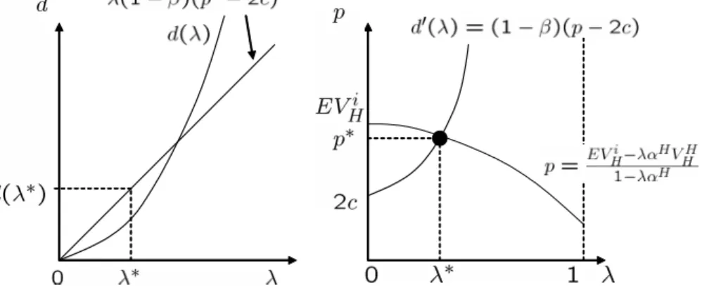
conditional on knowing λ∗. Sufficiently low γ leads to low λ∗, resulting in the somewhat low equilibrium price p∗, then the informed L=buyer accepts the price once he knows that the product quality is definitely H. Clearly, the H-seller also accepts the price. However, price p∗ is still too high for the L-buyer to accept, even if he knows that the product quality is definitely M . Consequently, IA does not increase a probability of trading for the M -seller; thus, the M -seller does not use IA. Note that the equilibrium price in the case IA is lower than the equilibrium price in the benchmark case, because the uninformed L-buyer correctly calculates the expected quality as lower in the case IA. Figure 1 shows p∗ and λ∗.
Figure 1 Equilibrium probability and equilibrium price in the case IA
3.3 Uninformative Advertising
We consider a PBE of the game where only UA is available (case UA). The seller may distinguish herself from the other lower types of sellers by using UA. The seller is required to create a sufficiently high level of UA that the buyer believes the product quality is high. Thus, whether the seller uses UA depends crucially on both the buyer’s belief and the difference among cost functions of UA (ei), and multiple equilibria exist unlike the benchmark case or the case IA. As we will see below, the different types of sellers offer different prices if and only if they choose different levels of UA.
Proposition 3 (case UA) There are two semi-separating PBEs with UA and one pooling PBE with UA.
(1) The following semi-separating PBE exists. In equilibrium, the H-seller offers price p = VHH, while both the M -seller and the L-seller offer p = α
MVHM+αLVHL
αM+αL . Only the H-buyer accepts the prices. Only the H-seller uses UA by choosing a level ˆkgiven by:
³
eL´−1³β³VHH −α
MVM
H + αLVHL
αM + αL
´´≤ ˆk≤³eH´−1³β³VHH −α
MVM
H + αLVHL
αM + αL
´´ . The buyer’s belief is given by:
µ(θS|k, p) =
((0, 0, 1) if p ≥ VHH, k≥ ˆk (αMα+αL L,αMα+αM L,0) otherwise.
(2) The following semi-separating PBE exists. In equilibrium, both the H-seller and the M - seller offer price p = αHVαHHH+α+αMMVHM, while the L-seller offers price p = VHL. The H-buyer accepts the prices. Both the H-seller and the M -seller use UA by choosing a level ˜kgiven by:
³
eL´−1³β³ α
HVH
H + αMVHM
αH + αM − V
L H
´´
≤ ˜k≤³eH´−1³β³ α
HVH
H + αMVHM
αH+ αM − V
L H
´´ . The buyer’s belief is given by:
µ(θS|k, p) =
((0,αHα+αMM,αHα+αHM) if p ≥ αHVαHHH+α+αMMVHM, k≥ ˜k
(1, 0, 0) otherwise.
(3) The following pooling PBE exists. In equilibrium, all types of sellers offer price p = EVHi, and the H-buyer accepts the price. All types of sellers use UA by choosing a level ¯k given by:
0 < ¯k≤ (eL)−1(β(EVHi − VHL)).
The buyer’s belief is given by:
µ(θS|k, p) =
((αL, αM, αH) if p ≥ EVHi, k≥ ¯k (1, 0, 0) otherwise.
UA may or may not work as a signal of higher quality depending on the buyer’s belief. The buyer’s pessimistic belief that no advertising definitely implies the lowest quality supports the pooling PBE (3). In the PBE, all types of sellers choose the same level of UA and offer the same price. The cost of UA is the most severe to the L-seller, but the L-seller cannot benefit from quitting UA and offering a price that is acceptable to the H-buyer. Thus, the L-seller also uses UA. In this case, UA does not serve as a signal of higher quality. Note that the price offered in the PBE is the same as the price offered in the benchmark case; thus, all types of sellers’ profits are lower in the PBE compared with the benchmark case because of the cost of UA. Such a case is actually observed. Caves and Green (1996) found no evidence of correlation between product quality and prices and advertising outlays in their empirical study using consumer reports.
In the semi-separating PBE, however, UA serves as a signal of higher quality.11 In the semi-separating PBE (1), UA completely serves as a signal of higher quality. Given the buyer’s belief, the desirable level of UA is too high for both the M -seller and the L-seller to use UA, and thus the only the H-seller uses UA, convincing the buyer that the seller who chooses ˆk >0 and use UA is definitely a high type.
In the semi-separating PBE (2), UA partially serves as a signal of higher quality. Given the buyer’s belief, the desirable level of UA is lower in the PBE (2) than the PBE (1). Thus, both the H-seller and the M -seller choose the same level of UA, and then choose the same price. 3.4 Informative Advertising and Uninformative Advertising
In this subsection, we characterize a PBE with both IA and UA in a game where both IA and UA are available to the seller. As we will see below, there are multiple PBEs with both IA and
11If we allow the buyer’s belief that has two cutoff points, there exists a separating PBE whose outcome is given by each i-seller choosing a level of UA, kH > kM > kL= 0, and offering price pi = VHi. The following buyer’s belief is consistent with the seller’s strategy: µ∗(θS|k, p) = (0, 0, 1) if k ≥ kH and p ≥ pH, (0, 1, 0) if kH> k≥ kM and pH> p≥ pM and (1, 0, 0) otherwise.
UA. We are especially interested in a PBE where at least one type of seller combines IA with UA because we may capture some synergy effects of the advertising mix in such a PBE.
Proposition 4 (Case IU) There are two semi-separating PBEs with IA and UA, and one pooling PBE with IA and UA.
(1) Suppose γ ≤ ˆγ. The following semi-separating PBE exists. In equilibrium, the H-seller offers p = VHH, while both the M -seller and the L-seller offer p = ˆp. Only the M -seller chooses λ >ˆ 0 and uses IA:
λˆ= (1 − β)(ˆp− c) γ , pˆ=
(1 − ˆλ)αMVHM + αLVHL (1 − ˆλ)αM + αL , ˆγ=
(1 − β)(VLM − c)
λˆ .
The uninformed H-buyer, the informed H-buyer and the informed L-buyer accept the price p= ˆp, while only the H-buyer accepts p = VHH. Only the H-seller chooses ˆk >0 and uses UA:
Kˆ ≤ ˆk≤³eH´−1³β(VHH − ˆp) −(1 − β)
2(ˆp− 2c)2
2γ
´ ,
where
Kˆ = maxn(eL)−1(β(VHH − ˆp), ³eM´−1³β(VHH − ˆp) −(1 − β)
2(ˆp− 2c)2
2γ
´o . The buyer’s belief is given by:
µ(θS|k, p) =
(0, 0, 1) if p ≥ VHH, k≥ ˆk ( αL
(1−ˆλ)αM+αL,
(1−ˆλ)αM
αM+αL ,0) otherwise.
(2) Suppose γ ≤ ˜γ. The following semi-separating PBE exists. In equilibrium, both the H- seller and the M -seller offer price p = ˜p, while the L-seller offers price p = VHL. Only the H-seller chooses ˜λ >0 and use IA:
˜λ= (1 − β)(˜p− 2c) γ , p˜=
(1 − ˜λ)αHVHH+ αMVHM (1 − ˜λ)αH+ αM , γ˜=
(1 − β)(VLH − 2c)
˜λ .
The uninformed H-buyer, the informed H-buyer and the informed L-buyer accept the price p= ˜p, while only the H-buyer accepts p = VHL. Only the H-seller chooses ˜k >0 and uses UA:
(eL)−1(β(˜p− VHL)) ≤ ˜k≤³eM´−1³β(˜p− VHL) −(1 − β)
2(VL H − c)2
2γ
´ .
The buyer’s belief is given by:
µ(θS|k, p) =
(0, αM
(1−˜λ)αH+αM,
(1−˜λ)αH
(1−˜λ)αH+αM) if p ≥ ˜p, k≥ ˜k
(1, 0, 0) otherwise.
(3) The following pooling PBE exists. In equilibrium, all types of sellers offer price p = ¯p. Only the H-seller chooses ¯λ >0 and uses IA:
¯λ= (1 − β)(¯p− c) γ , p¯=
EVHi − ¯λαHVHH 1 − ¯λαH , γ¯=
(1 − β)(VLH− 2c)
λ¯ .
The uninformed H-buyer, the informed H-buyer and the informed L-buyer accept the price p= ˆp, while only the H-buyer accepts p = VHH. All types of sellers choose ¯k >0 and use UA:
0 < ¯k≤ minn(eL)−1(β(¯p− VHL)), ³eM´−1³β(¯p− VHL) − (1 − β)
2(VL H − c)2
2γ
´o.
The buyer’s belief is given by: µ(θS|k, p) =
((αL, αM, αH) if p ≥ EVHi, k≥ ¯k (1, 0, 0) otherwise.
As in the previous subsection, UA may or may not serve as a signal of higher quality, and thus there are three equilibrium outcomes. In the first semi-separating equilibrium (PBE (1)), UA completely serves as a signal of higher quality. Given the buyer’s belief, the desirable level of UA is too high for both the M -seller and the L-seller to mimic the H-seller. The seller can perfectly distinguish herself from lower types through UA, thus she has no longer incentives to use IA. However, the price offered by both the M -seller and the L-seller is relatively low for the informed L-buyer, and the informed L-buyer accepts the price if he definitely faces the M -seller, thus the M -seller can increase her demand by using IA. Both types of buyers construct a similar belief to the belief in the first semi-separating equilibrium of the case UA. Both types of uninformed buyers infer that the product quality is either medium or low unless they observe a high level of UA and face the high price. On not receiving IA, however, both types of uninformed buyers evaluate the expected valuation lower than the case UA, because they cannot distinguish between the case in which the seller’s type is low and she does not distribute IA, and the case in which the seller’s type is medium but the buyer does not receive IA.
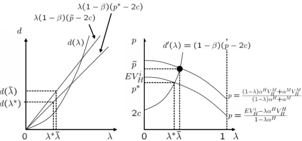
Figure 2 Equilibrium probability and equilibrium price in the semi-separating PBE (2) of the case IU
In the second semi-separating equilibrium (PBE(2)), UA serves as a partial signal of higher quality. As previously, the desirable level of UA is too high for the L-seller to use. Similar to the case IA, the H-seller can increase her demand by using IA, thus she uses IA. The price offered by both the H-seller and the M -seller seems low for the L-buyer to accept if he knows that the product quality is definitely high. Both types of uninformed buyers infer that the product quality is definitely low unless they observe the high level of UA and face the high price. On not receiving IA, however, both types of uninformed buyers evaluate the expected valuation lower than the case UA.
In the pooling equilibrium (PBE (3)), UA does not serve as a signal of higher quality, but all types of sellers use UA and offer the same price. While UA seems somewhat redundant, both types of buyers infer that the product quality is definitely low, conditional on not observing UA, thus all types of sellers are forced to use UA. The H-seller also uses IA, increasing her demand, because the equilibrium price is lower than the L-buyer’s willingness to pay conditional on knowing that the product quality is high, resulting in the price to be accepted by the H- buyer and the informed L-buyer. Both types of buyers construct a similar belief to the belief in the pooling equilibrium of the case UA. Notice that both the equilibrium price ¯p and the equilibrium proportion of informed buyers ¯λare the same values as in the PBE of the case IA.
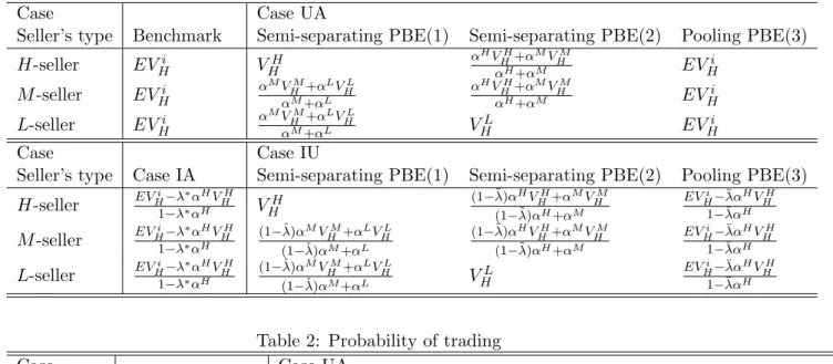
Table 1: Equilibrium prices
Case Case UA
Seller’s type Benchmark Semi-separating PBE(1) Semi-separating PBE(2) Pooling PBE(3)
H-seller EVHi VHH α
HVH H+α
MVM H
αH+αM EV
i H
M-seller EVHi α
MVM H+αLVHL αM+αL
αHVHH+αMVHM
αH+αM EV
i H
L-seller EVHi α
MVM H+αLVHL
αM+αL V
L
H EVHi
Case Case IU
Seller’s type Case IA Semi-separating PBE(1) Semi-separating PBE(2) Pooling PBE(3) H-seller EVHi1−λ−λ∗∗ααHHVHH VHH (1−˜λ)α
HVH H+α
MVM H
(1−˜λ)αH+αM
EVHi−¯λαHVHH 1−¯λαH
M-seller EVHi1−λ−λ∗∗ααHHVHH
(1−ˆλ)αMVHM+αLVHL (1−ˆλ)αM+αL
(1−˜λ)αHVHH+αMVHM (1−˜λ)αH+αM
EVHi−¯λαHVHH 1−¯λαH
L-seller EV
i H−λ
∗αH
VHH 1−λ∗αH
(1−ˆλ)αMVHM+αLVHL
(1−ˆλ)αM+αL V L H
EVHi−¯λαHVHH 1−¯λαH
Table 2: Probability of trading
Case Case UA
Benchmark Semi-separating PBE(1) Semi-separating PBE(2) Pooling PBE(3)
Probability β β β β
Case Case IU
Case IA Semi-separating PBE(1) Semi-separating PBE(2) Pooling PBE(3) Probability β+ λ∗(1 − β)αH β+ ˆλ(1 − β)αM β+ ˜λ(1 − β)αH β+ ¯λ(1 − β)αH
4 Results
In this section, we consider contributions of IA and UA on probability of trading and revenue.
Informative advertising Because the probability of the buyer being a high type is suffi- ciently large (β ≥ ¯β), all types of sellers want to offer the high price acceptable to only the H-buyer, leading to pooling equilibria in both the benchmark case and the case IA. How- ever, the equilibrium price is lower in the case IA (p = EVHi) than in the benchmark case (p = EV
i H−λ∗α
HVH H
1−λ∗αH ). This is because, conditional on not receiving IA, the probability of the product quality being high is lower than the initial probability αH. Thus, IA alone decreases the equilibrium price. However, IA alone raises the probability of trading for the H-seller who
uses IA in equilibrium, because the H-seller can trade with the informed L-buyer in addition to the H-buyer. Furthermore, it is ambiguous whether the H-seller obtains a higher profit in the case IA than in the benchmark case. If the cost of IA is sufficiently low, i.e., γ is suf- ficiently small, then the H-seller benefits from using IA. Both the M -seller and the L-seller trade with only the H-buyer in both cases, and they obtain a lower profit in Case IA than in the benchmark case. We summarize this observation as Proposition 5.
Proposition 5 IA alone increases the ex ante probability of trading but decreases the price. Neither the M -seller nor the L-seller obtains a higher profit in the case IA than in the benchmark case. There exists an upper bound ¯γ, and the H-seller obtains a higher profit in the case IA than in the benchmark case if and only if γ ≤ ¯γ, such that:
¯
γ = (1 − β)
2(p∗∗− 2c)2
2β(p∗− p∗∗) .
In addition, as pointed out in Moraga-Gonzalez (2000), the optimal level of IA (λ) increases in the equilibrium price, because λ is determined at a level where the seller’s marginal revenue is equivalent to the marginal cost of using IA; i.e., d′(λ) = (1 − β)(p − ci), where the left-hand side is the marginal cost and the right-hand side is the marginal revenue for the i-seller. The intuition is that high prices are likely to discourage the L-buyer who does not receive IA, and the H-seller raises the level of IA in order to sell the product to the L-buyer. In contrast to Proposition 5, Moraga-Gonzalez (2000) shows that the equilibrium price of a non-advertising pooling equilibrium is lower than the equilibrium price of an advertising pooling equilibrium. In an actual business setting, however, low prices in sales promotion may be necessary to enhance IA (sampling) (Scott (1976)).
Uninformative advertising There exist multiple equilibria where UA is used, two semi- separating PBEs and one pooling PBE, depending on the buyer’s belief. Furthermore, UA works as a perfect/partial signal of product quality in the two semi-separating PBEs, while UA does not provide any information on the product quality to the buyer in the pooling PBE. Some empirical studies find that advertising outlays serve as a signal of higher product quality
(Tellis and Fornell (1988), Nichols (1998)), while the others show that no positive relationship exists between advertising outlays and the product quality (Caves and Greene (1996)).
In the first semi-separating PBE, only the H-seller uses UA, and UA works as a perfect signal of the highest quality. The H-seller offers a higher price p = VHH in the case UA than in the benchmark case, while both the M -seller and the L-seller offer a lower price in the case UA than in the benchmark case. In the second semi-separating PBE, both the H-seller and the M-seller use UA, and UA works as a partial signal of higher quality. The prices are lower in the case UA than the equilibrium price in the benchmark case. In the pooling PBE, all types of sellers use UA, which does not work as a signal of higher quality. All types of sellers offer the same price as the equilibrium price in the benchmark case.
The three equilibria imply that UA does not decrease the equilibrium prices for the seller who uses UA. In particular, if UA serves as a (partial) signal of higher quality, then using UA increases the equilibrium prices. However, all the equilibrium prices in the case UA are accepted by only the H-buyer as in the benchmark case. Thus, using UA has no effect on the probability of trading.
Regarding the expected profit, there may exist cases where the case UA earns the seller higher expected profits than the benchmark. If there is a big gap of costs of UA among types of sellers, for certain level of UA, then using UA imposes very few costs on the seller who uses UA, leading to the higher expected profits. Actually, the H-seller can obtain the higher expected profits in the case UA than the benchmark. However, neither the M -seller nor the L-seller obtains a higher profit in the case UA than in the benchmark case. We summarize this observation as Proposition 6.
Proposition 6 UA alone increases the equilibrium prices but has no effect on the ex ante probability of trading. Neither the M -seller nor the L-seller obtains a higher profit in the case UA than in the benchmark case. The H-seller obtains a higher profit in the case UA (the second semi-separating PBE) than in the benchmark case if there is a big gap of costs of UA among types of sellers.
Informative advertising and uninformative advertising There exist multiple equilibria where both IA and UA are used, two semi-separating PBEs and one pooling PBE, depending on the buyer’s belief, such as the PBE of the case UA.
In the first semi-separating PBE, where UA works as a perfect signal of the highest quality, IA and UA are separately used. Only the H-seller uses UA, while only the M -seller uses IA. By comparing the semi-separating PBEs in the case IU with the PBE in the benchmark, we observe the following: IA increases a probability of trading but decreases a price, while UA increases a price but has no effect on a probability of trading, as previously.
In the pooling PBE, there is no effect of UA that increases a price because UA does not serve as a signal of higher quality, but there is still on effect of IA that decreases a price, thus the equilibrium price is strictly lower in the case IU than the benchmark. Actually, the equilibrium price is the same as that in the case IA. In this case, we find no effect of advertising mix, i.e., the H-seller uses both IA and UA.
As we will see below, there exists a positive synergy effect of advertising mix in the second semi-separating PBE.
Synergy effect As we saw above, UA alone does not increase the probability of trading. By combining UA with IA, however, UA can increase the probability of trading. The reason is as follows. If the seller uses IA and offers a price acceptable to the H-buyer and the informed L-buyer, the probability of trading is given by β +λ(1−β), given the level of IA λ. The optimal level of λ increases in price p in equilibrium, and the signaling effect through UA raises the equilibrium price. Notice that λ increases in p because of d′ >0 and d′′>0. This is an indirect effect of UA that increases the probability of trading through an increase of the price. The indirect effect of UA is a source of a synergy effect of the advertising mix ; that is, UA increases both the price and the probability of trading whenever the seller uses IA. In fact, the H-seller can trade with a probability β + ˜λ(1 − β) in the second semi-separating PBE in the case IU, while β + ¯λ(1 − β) in the PBE in the case IA, where β + ˜λ(1 − β) > β + ¯λ(1 − β). However, neither the M -seller nor the L-seller combines UA with IA, and they do not enjoy the synergy effect of the advertising mix. We summarize the above observation as Proposition 7.
Proposition 7 (Synergy effect) There exists a synergy effect of the advertising mix because of the indirect effect of UA where UA indirectly increases the probability of trading through an increase of the price whenever the seller uses IA. The H-seller enjoys the synergy effect, while neither the M -seller nor the L-seller enjoys the synergy effect.
Three points are worth noting here. First, only the H-seller can enjoy the synergy effect of the advertising mix. IA needs the fact that the product quality is sufficiently high. Even though the M -seller and the L-seller use IA, the informed L-buyer does not buy the product; therefore, they cannot enjoy the synergy effect of the advertising mix. Second, the synergy effect vanishes as the probability of the L-buyer decreases. If no L-buyer exists, the seller cannot increase the probability of trading by using IA; thus, the synergy effect disappears. We obtain ¯λ→ 0 and ˜λ → 0 as β → 1. Furthermore, the equilibrium prices are approaching to p= EVHi as β → 1. Third, a partial signal of higher quality is the source of the synergy effect. If UA does not work as a signal of higher quality at all (pooling PBE), UA does not increase the price; therefore, the synergy effect is not realized. However, if UA works as a perfect signal of higher quality, the synergy effect is not realized either. In the case of the perfect signal, the buyer knows the product quality completely; therefore, IA is redundant.
We can interpret Proposition 7 as follows. If the H-seller airs excellent (or many) TV commercials, the brand of her product becomes well known to consumers, and then consumers are likely to receive and try free samples. As a consequence, the consumers learn of the high product quality and buy the products.
In the economics literature, many studies have discussed the function of UA as a signal of higher product quality in informative view (Bagwell (2003)). In addition to the signaling function, Proposition 7 gives the other function of UA.
In the marketing literature, many studies point out that prior advertising can raise the trial rate, which is the proportion of consumers who use the free samples (Heiman et al. (2001)), and the positive effect of advertising on sampling (IA) is confirmed in experiments (Kempf and Smith (1998), Kempf and Laczniak (2001)).
5 Discussion
Many buyers We can easily extend our model to the case where there are a large number of buyers. A parameter β is a proportion of buyers who are highly interested in the product. Each buyer has a unit demand. In such a case, the results do not change at all, but we may interpret advertising differently. When the seller uses IA, she chooses λ > 0 as a ratio of the targeted buyers. The high ratio λ implies distributing free samples widely, imposing the high promotion cost on the seller.
Three types of sellers In our mode, the buyer has two types, while the seller has three types. If we adopt two types of sellers, say, H and L, then the results dramatically change. In such a case, the equilibrium where one type of sellers use both IA and UA and UA serves as a signal of higher quality disappears, vanishing the effect of advertising mix. The reason is the followings. If only the H-seller uses UA, then the buyer can perfectly know the seller’s types, and thus IA is redundant to the seller. Therefore, in any equilibrium with both IA and UA, both the H-seller and the L-seller must use UA, which does not serve as a signal of higher product quality. Therefore, the assumption of three types of sellers is important. However, the results will remain for more than three types of sellers and two types of buyers, though multiple cases will arise, making results much more complex.
Internal solutions of λ We assumed internal solutions for optimal probabilities of the buyer to be informed, 0 < λ < 1, i.e., the seller cannot choose λ = 1 because of huge costs of IA. However, if the seller could choose λ = 1 and use IA with sufficiently low cost, then she would never use UA since the costly UA is redundant. Therefore, the equilibrium that brings the H-seller the synergy effect of advertising mix would vanish. Furthermore, in the case IU, there should exist a unique equilibrium where both the H-seller and the M -seller should use IA and no types of sellers use UA, which is separating. In the sense that the seller can definitely distinguish herself from lower types, IA is aways preferred to UA if λ = 1 can be chosen by the seller. In practice, however, choosing λ = 1 implies that the seller distributes free samples to all consumers, seems fantastic.
6 Conclusion
We considered a market under bilateral asymmetric information and analyzed two tools for advertising product quality. The first is informative advertising (IA), such as distributing free samples, which conveys the actual product quality to the buyer. The second is uninformative advertising (UA), such as airing TV commercials, which serves as a signal of high product quality. Both tools can serve to advertise the product quality, but they have different effects. IA increases the probability of trading by conveying the high product quality to the buyer with the low valuation but decreases the price by lowering the expected valuation of the uninformed buyer who does not receive the IA. However, UA increases the price by making the buyer’s belief high but does not change the probability of trading. We find an equilibrium where combining IA with UA increases the probability of trading. UA raises the equilibrium price, leading that the seller optimally chooses the high probability of the buyer to be informed. As a result, the probability of trading increases. This is the synergy effect of the advertising mix, i.e., combining IA with UA, and only a partial signal of the product quality is needed for the synergy effect. The result sheds light on a new function of UA.
We considered three types of sellers and two types of buyers. An analysis that includes three types of sellers may seem somewhat strange, while two types is common. However, if there exist only two types of sellers, the equilibrium with the synergy effect (PBE (2) of the case IU) vanishes, and thus the analysis becomes less interesting. We considered only two marketing activities here, but we can allow other marketing methods for the seller. For example, the seller can undertake costly investment to increase the product quality. We can extend our model and analyze several marketing mixes. These topics will be future research issues.
7 References
1. Akerlof, G.A. “The Market for ‘Lemons’: Quality Uncertainty and the Market Mecha- nism”, Quarterly Journal of Economics, Vol.84 (1970), pp.488–500.
2. Bawa, K. and Shoemaker, R. “The Effects of Free Sample Promotions on Incremental Brand Sales”, Marketing Science, Vol.23, No.3, (2004), pp.345–363.
3. Caves, R.E. and Green, D.P. “Brands’ Quality Levels, Prices and Advertising Outlays: Empirical Evidence on Signals and Information Costs”, International Journal of Indus- trial Organization, Vol.14 (1996), pp.29–52.
4. Chatterjee, K. and Samuelson, W. “Bargaining under Incomplete Information”, Opera- tions Research, Vol.31 (1983), pp.835–851.
5. Fudenberg, D. and Tirole, J. “Sequential Bargaining with Incomplete Information”, Re- view of Economic Studies, Vol.2 (1983), pp.221–247.
6. Tellis, G.J. and Fornell, C. “The Relationship between Advertising and Product Quality over the Product Life Cycle: A Contingency Theory”, Journal of Marketing Research, Vol.25 (1988), pp.64–71.
7. Heiman, A., McWilliams, B., Shen, Z. and Zilberman, D. “Learning and Forgetting: Modeling Optimal Product Sampling over Time”, Management Science, Vol.47, No.4, (2001), pp.532–546.
8. Horstmann, I. and MacDonald, G. “When Is Advertising a Signal of Product Quality?”, Journal of Economics and Management Strategy, Vol.3 (1994), pp.561–584.
9. Horstmann, I. and MacDonald, G. “Is Advertising a Signal of Product Quality? Evidence from the Compact Disk Player Market, 1983–1992”, International Journal of Industrial Organization, Vol.21 (2003), pp.317–345.
10. Kihlstrom, R.E. and Riordan, M.H. “Advertising as a signal”, Journal of Political Econ- omy, Vol.92 (1984), pp.427–450.
11. Mailath, G.J., Okuno-Fujiwara, M., and Postlewaite, A. “Belief-Based Refinements in Signaling Games”, Journal of Economic Theory, Vol.60 (1993), pp.241–276.
12. Milgrom, P. and Roberts, J. “Price and Advertising Signals of Product Quality”, Journal of Political Economy, Vol.94 (1986), pp.796–821.
13. Moraga-Gonzalez, J.L. “Quality Uncertainty and Informative Advertising”, International Journal of Industrial Organization, Vol.18 (2000), pp.615–640.
14. Myerson, R. and Satterthwaite, M. “Efficient Mechanisms for Bilateral Trading”, Journal of Economic Theory, Vol.29 (1983), pp.265–281.
15. Nelson, P. “Information and Consumer Behavior”, Journal of Political Economy, Vol.78 (1970), pp.311–329.
16. Nelson, P. “Advertising as Information”, Journal of Political Economy, Vol.82 (1974), pp.729–754.
17. Nichols, M.W. “Advertising and Quality in the U. S. Market for Automobiles”, Southern Economic Journal, Vol.64(4) (1998), pp.922–939.
18. Shavell, S. “Acquisition and Disclosure of Information prior to Sale”, The RAND Journal of Economics, Vol.25 (1994), pp.20–36.
19. Tsuchihashi, T. “Market Research and Complementary Advertising under Asymmetric Information”, Hitotsubashi University discussion paper No.2008-5 (2008), pp.1–31.
8 Appendix
Proof of Proposition 1
Proof. Let B(p) be a conditional probability of price p to be accepted. Since both types of buyers have the same belief, the H-buyer accepts the price whenever the L-buyer accepts the price; thus, we have B(p) ∈ {0, β, 1}.
First, we show that any equilibrium must be pooling. Suppose that there exists a semi- separating equilibrium. Denote by pi an equilibrium price that the i-seller offers. Monotone belief ensures pH ≥ pM ≥ pL, resulting in B(pH) ≤ B(pM) ≤ B(pL), since the M -seller benefits from mimicking the H-seller’s price if B(pH) > B(pM), and so on. If pH > pM > pL, then B(pH) = 0 should hold, giving the H-seller a profitable deviation. We separately consider two cases: (1) pH = pM > pL and (2) pH > pM = pL.
The case (1) B(pH) = B(pM) = β < B(pL) = 1 must hold, thus the prices are given by pH = pM = α
HVH H+α
MVM H
αH+αM and pL = VLL. In such a case, however, the L-seller benefits from