C209 2009 11 WRTLT 最近の更新履歴 Hideo Fujiwara

(1)

Observation-Point Selection at the Register-Transfer Level to

Enhance Defect Coverage for Functional Test Sequences ^∗

Hongxia Fang¹, Krishnendu Chakrabarty¹ and Hideo Fujiwara²

1ECE Dept., Duke University, Durham, NC, USA ²Nara Institute of Science and Technology, Nara, Japan

Abstract— Functional test sequences for manufacturing test are typically derived from test sequences used for design verification. Since long verification test sequences cannot be used for manufacturing test due to test-time constraints, functional test sequences often suffer from low defect coverage. In order to increase their effectiveness, we propose a DFT method that uses the register-transfer level (RTL) output- deviations metric to select observation points for an RTL design and a given functional test sequence S. The selection of observation points is based on the output deviation for S and the topology of the design. Simulation results for six ITC’99 circuits and the OpenRisc1200 CPU show that the proposed method outperforms two baseline methods in terms of the stuck-at and transition fault coverage, as well as for two gate-level defect coverage metrics, namely bridging (BCE+) and gate- equivalent fault coverage. Moreover, by inserting a small subset of all possible observation points using the proposed method, significant defect coverage increase is obtained for all benchmark circuits.

I. INTRODUCTION

Structural test for modeled faults at the gate level is widely used in manufacturing testing [1]. Although structural tests can be developed to achieve high fault coverage for modeled faults, they often suffer from inadequate defect coverage. Scan-based structural testing for aggressive defect screening is also associated with the problems of overtesting and yield loss [2] [3]. Hence functional tests are often used to supplement structural tests to improve test quality [4] [5]. However, it is impractical to generate and evaluate functional test sequences at gate-level for large circuits. A more practical alternative is to carry out test generation, test-quality evaluation, and design-for-testablity (DFT) earlier in the design cycle at the register-transfer (RT) level [6]–[9].

A number of methods have been presented in the literature for test generation at RT-level [10]–[16]. However, they usually suffer from low gate-level fault coverage due to the lack of gate-level information or due to the poor testability of the design. To increase testability and to ease test generation, various DFT methods at RT-level have also been proposed. These DFT methods can be classiﬁed into two categories, namely scan-based methods [17]–[21] and techniques that do not use scan design [22]–[27]. Scan-based DFT techniques are easy to implement, but they lead to long test application time and they are less useful for at-speeding testing. Non-scan DFT techniques offers lower test application time and they facilitate at-speed testing. In [22], non-scan DFT techniques are proposed to increase the testability of RT-level designs. The orthogonal scan method, which uses functional datapath ﬂow for test data, is proposed in [23] to reduce test application time. In [24] [25], design-for-hierarchical-testability techniques were described to aid hierarchical test generation. In [26], the authors presented a method based on strong testability, which exploits the inherent characteristic of datapaths to guarantee the existence of test plans (sequences of control signals) for each hardware element in the datapath. To reduce the overhead associated with strong testability, a linear-depth time-bounded DFT method was presented in [27].

∗This research was supported in part by the Semiconductor Research Corporation under Contract no. 1588, and by an Invitational Fellowship from the Japan Society for the Promotion of Science.

Although much work has been done on RTL DFT to increase testability and ease RT-level test generation, much less work on RTL DFT has been targeted towards increasing the defect coverage of existing functional test sequences. The generation of functional test sequences is a particularly challenging problem, since there is insufficient automated tool support and this task has to be accomplished manually or at best in a semi-automated manner. Therefore, functional test sequences for manufacturing test are often derived from design-verification test sequences [28]–[30] in practice. It is impractical to apply such long verification sequences during time-constrained manufacturing testing. Therefore, shorter subsequences must be used for testing, and this leads to the problem of inadequate defect coverage. Therefore, we focus on RTL DFT to increase the effectiveness of these existing test sequences.

To enhance the effectiveness of given test sequence for an RT-level design, we can either insert control points to increase the controllability of the design or observation points to increase the observability of the design. In this work, we limit ourselves to the selection and insertion of observation points. We use the RT-level output deviation metric from [31] and the topology information of the design to select and insert the most appropriate observation points. The RT-level output deviation metric has been deﬁned and used in [31] to grade functional test sequences.

To evaluate the proposed observation-point selection method, we use sixIT C^′99 circuits as well as the OpenRISC 1200, which is more representative of industry designs, as the experimental vehicles. Simulation results show that the proposed method outperforms two baseline methods for defect coverage (represented by gate-level bridging and gate-equivalent fault coverage, as well as traditional stuck-at and transition fault coverage). Moreover, by inserting a small subset of all possible observation points using the proposed method, signiﬁcant defect coverage increase is obtained for all circuits.

The remainder of this paper is organized as follows. Section II deﬁnes the problem and presents the proposed observation- point selection method based on RT-level deviations and topology information. The design of experiments and experimental results are reported in Section III. Section IV concludes the paper.

II. OBSERVATION-POINT SELECTION

In this section, we first define the DFT problem being tackled in this paper. Next we give basic definitions for topology. Then we introduce the new concept of RT-level internal deviations. Following this, we introduce the metrics that can be used to guide observation-point selection. Finally, we present the observation- point selection algorithm based on RT-level output deviations and topology information of the design.

A. Problem deﬁnition

To make the existing functional test sequences more useful for targeting defects in manufacturing testing, we can increase the testability of the design by inserting an observation point for each 10th IEEE Workshop on RTL and High Level Testing (WRTLT'09), pp. 16-22, Nov. 2009.

(2)

Reg0

Reg1 Reg4

Reg3 Reg6

Reg2 _Reg5 _Reg7

PI1

PO1

PO2

Fig. 1. An example to illustrate RTL topology.

register output. However, it is impractical to insert all possible observation points since it will lead to high hardware and timing overhead. In practice, the number of observation points is limited by area and performance considerations. For a given upper limit n, our goal is to determine the best subset of n observation points from all the possible observation points such that we can maximize the defect coverage, i.e., maximize the effectiveness, of a given functional test sequenceS. When n is not given, another interesting problem arises: Given RT-level description for a design and a functional test sequence S and given the highest fault coverage that can be obtained byS and by inserting the maximum number of observation points, the goal is to determine both n and n observation points to maximize the effectiveness ofS. In this paper, we focus on the ﬁrst case when n is given. For the second case, we will investigate it in the future work.

B. Topology analysis

We exploit RTL topology information, which refers to the interconnection between registers and combinational blocks at RT- level; see Fig. 1. Each oval in Fig. 1 represents a register while each

“cloud” represents a combinational block between two registers. A directed edge implies possible dataﬂow. From the extracted topology graph G, we can see how registers are connected to each other through combinational blocks. We next deﬁne related terminology that is used in the paper.

1-level downstream and upstream registers: Consider two reg- isters R1 and R2. If there is a directed edge from R1 to a combinational block in G, and there is a directed edge from the same combinational block toR2, thenR2 is a1-level downstream register forR1(denoted asR2D R1) andR1is a1-level upstream register forR2 (denoted asR1 U R2). For example, in Fig. 1, we haveR3 D R0 andR0 U R3.

p-level downstream and upstream registers (p>1): This is a recursive deﬁnition and it is based on the 1-level downstream register and upstream register deﬁned above. Consider two registers R1 andRp+1. If there is a sequence of registersRi (i = 2..., p) such that(R2 D R1)^!...(Ri+1 D Ri)^!...(Rp+1 D Rp) is true, and if Rp+1 is not a k-level downstream register for R1 (k < p), then Rp+1 is a p-level downstream register for R1 and Rp+1 is a p-level upstream register for R1. For example, in Fig. 1, Reg7 is a 3-level downstream register for Reg0 and Reg0 is a 3-level upstream register forReg7.

C. RT-level internal deviations

The RT-level output deviation forS has been deﬁned in [31] to be a measure of the likelihood that error is manifested at a primary output. It can be calculated at RT-level for a given design based

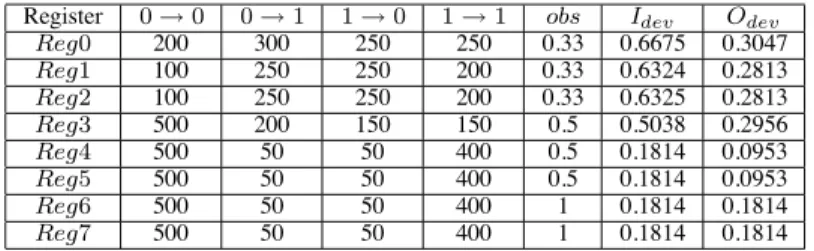
TABLE I. Difference between internal deviations and output deviations. Register 0 → 0 0 → 1 1 → 0 1 → 1 obs Idev Odev

Reg0 200 300 250 250 0.33 0.6675 0.3047

Reg1 100 250 250 200 0.33 0.6324 0.2813

Reg2 100 250 250 200 0.33 0.6325 0.2813

Reg3 500 200 150 150 0.5 0.5038 0.2956

Reg4 500 50 50 400 0.5 0.1814 0.0953

Reg5 500 50 50 400 0.5 0.1814 0.0953

Reg6 500 50 50 400 1 0.1814 0.1814

Reg7 500 50 50 400 1 0.1814 0.1814

on three contributors. The ﬁrst contributor is the transition count (TC) of registers. Higher the TC for a functional test sequences, the more likely is it that this functional test sequences will detect defects. The second contributor is the observability of a register. The TC of a register will have little impact on defect detection if its observability is so low that transitions cannot be propagated to primary outputs. Therefore, each output of registers is assigned an observability value using a SCOAP-like measure. The third contributor to RT-level output deviation is the weight vector, which is used to measure how much combinational logic a register is connected to. Each register is assigned a weight value, representing the relative sizes of its input cone and fanout cone.

Before analyzing the factors that determine the selection of observation points, we ﬁrst introduce the new concept of RT-level internal deviations. We deﬁne the RT-level internal deviation to be a measure of the likelihood of error being manifested at an internal register node, which implies that an error is manifested at one or more bits of register outputs. The calculation of RT-level internal deviations is different from that for RT-level output deviations, in that here we do not consider whether a transition in a register is propagated to a primary output.

We use an example to illustrate the difference between internal deviations and output deviations. Consider a circuit with the topology shown in Fig. 1. Suppose the CL vector is(1, 0.998, 0.998, 1). To simplify the calculation we suppose that the weight value for each register is1. Suppose that, for a functional test sequence T S, we have recorded the TCs of the registers for each type of transition in Columns2−5 of Table I. In the same table, the column obs shows the observability value of each register, which is obtained from the topology information.Idev andOdev list the internal deviation value and output deviation value for each register, respectively. For example, the internal deviation value of Reg0 is calculated as1 − 1^200·1· 0.998^300·1· 0.998^250·1· 1^250·1^{, i.e.,}0.6675. The output deviation ofReg0 is calculated as 1 − 1^200·1·0.33· 0.998^300·1·0.33· 0.998^250·1·0.33· 1^250·1·0.33, i.e.,0.3047.

D. Metrics to guide observation-point selection

Next we describe two RTL testability metrics that can be used for evaluating the quality of test sequences. We also show how these two metrics can be combined to guide the selection of observation- points for DFT. The ﬁrst metric is related to the output deviation for the test sequenceS while the second metric considers the topology of the RTL design.

1) RT-level output deviations: In this work, we only consider the insertion of observation points at outputs of registers. For a register Reg, we have the following attributes attached to it: Idev(Reg), Odev(Reg), obs(Reg). These attributes represent its internal deviation, output deviation, and observability value, respectively. For two registers Reg1 and Reg2, we deﬁne the following two observation-point-selection rules:

(3)

Rule 1: If Reg1 and Reg2 do not have predecessor/succssor relationship andIdev(Reg1) > Idev(Reg2), select Reg1;

Rule 2: When Reg1 is the logical predecessor of Reg2, and Idev(Reg1) is close in value with Idev(Reg2), select Reg2.

For Rule1, the motivation is that if we select a register with higher Idev, its observability will becomes1. Thus, its Odev will also become higher. The higher Odev of this register contributes more to Odev for the circuit. Since it has been shown that cumu- lativeOdev is a good surrogate metric for gate-level fault coverage [31], we expect to obtain better gate-level fault coverage when we select a register with higherIdev.

For Rule 2, if we select Reg2, obs(Reg2) will become 1 and obs(Reg1) will also be increased due to the predecessor relationship between Reg1 and Reg2. Therefore, it is possible that the selection of Reg2 yields better results than the selection of Reg1, i.e., the cumulative observability after the insertion of observation point onReg2 is higher than for Reg1.

To satisfy the above two rules, we consider the RT-level output deviations in guiding the selection of observation points. Since Odev is proportional toIdev and obs, if we select a register with higher Odev, we will tend to select the register with higher Idev

and higherobs. Therefore, we satisfy Rule 1 as well as implicitly satisfying Rule 2: for two registers Reg1 and Reg2 whose Idev

values are comparable, if Reg1 is the predecessor of Reg2, we have obs(Reg1) < obs(Reg2) and Odev(Reg1) < Odev(Reg2). Then we will not selectReg1, which is in accordance with Rule 2. 2) Topology information: The RT-level output deviation metric alone is not sufficient to ensure the selection of best observation points. If we select a register (labeled as R1) with the highest output deviation, it does not enhance the output deviation of its downstream registers. Instead, if the observation point is inserted a downstream of R1 (says R2), it benefits R1 as well as other registers betweenR1andR2. Therefore, selecting one register with the highest output deviations in each step does not always lead to the steepest increase in the overall output deviation value for the whole circuit. Let us revisit the example of Section II-C. The output deviation for the original circuit calculated using [31] is0.8612. If we want to select one observation point, according to theOdev of each register in Table I, we will selectReg0 since it has the highest output deviation value. The observability value of Reg0 will be increased to 1 and the observability value of all other registers will remain unchanged. Based on the updated observability vector, the overall output deviation value can be recalculated as 0.9336. The increase in output deviation is 0.9336 − 0.8612, i.e., 0.0724. However, if we considerReg3 (the 1-level downstream register of Reg0) as the observation point, the observability value of Reg3 is increased to 1 and the observability value of Reg0, Reg1, Reg2 will also be increased to0.5. The overall output deviation value will be calculated to be0.9423 and the increase in output deviation is 0.9423 − 0.8612 in this case, i.e., 0.0811. From the above example, we see that in some cases, the register with the highest output deviation is not the best choice for inserting an observation point. We therefore consider both the topology information and output deviation as metrics to guide observation-point selection. In each step, we consider k candidate registers (where k is a user-defined parameter) and evaluate the deviation improvement for the whole circuit for each of the k observation points. The best candidate is selected in each step. The k candidate registers are determined as follows. First, we take them registers with the

highest output deviations. Next, take1-level to p-level (p is set to 2 in this paper) downstream registers of these top-most deviation registers in order until the number of candidate registers reachesk. E. Observation-point selection procedure

In the selection of observation-points, we target the speciﬁc bits of a register. The calculation ofIdev,Odev,obs is carried out for each bit of a register. Given an upper limitn on the number of observation points, the selection procedure is as follows:

• Step0: Set the candidate set to be all bits of registers that do not directly drive a primary output.

• Step1: Derive the topology information for the design and save it in a look-up table. Obtain the weight vector, observability vector, and TCs for each register bit, and calculate RT-level output deviations for each register bit.

• Step2: Take m register bits with the highest output deviations. Take 1-level to p-level downstream register bits of these m top-most deviation register bits in order based on the topology information, until the number of these register bits reaching k. Put these k register bits in the current candidate list.

• Step 3: For each register bit in the current candidate list, evaluate the output deviation improvement for the design when it is inserted as an observation point. Select the best candidate and clear the current candidate list.

• Step4: If the number of selected observation points reaches n, terminate the selection procedure.

• Step 5: Update the observability vector using the inserted observation point (selected in Step 3) and the topology information. Re-calculate output deviations for each register bit using the updated observability vector. Go to Step2.

In Step 1, the topology information of the design, including all the direct predecessor bits and all the direct successor bits for a register bit, can be extracted using a design analysis tool, e.g., Design Compiler from Synopsys. It only needs to be determined once and it can be saved in a look-up table for subsequent use. In Step 3, each time we put k register bits in the current candidate list. These k register bits comes from register bits with top-most output deviations and their downstream register bits. In Step4, after selecting and inserting an observation point, we need to update the observability vector because the observability of its upstream nodes will also be enhanced. There is no need to recompute TCs and the weight vector since they depend only on the functional test sequence, and they are not affected by observation points.

III. EXPERIMENTAL RESULTS

To evaluate the efﬁciency of the proposed observation-point selection method, we performed experiments on sixIT C^′99 circuits [7] as well as on a more industry-like design, i.e., the OpenRISC 1200 processor [32]. The OpenRISC 1200 is a 32-bit scalar RISC with Harvard microarchitecture, 5-stage integer pipeline, virtual memory support (MMU), and basic digital signal processor (DSP) capabilities. The functional test sequences for the sixIT C^′99 are generated using the RT-level test generation method from [7]. For the OpenRISC 1200, the functional test sequences are obtained by simulation of the design-veriﬁcation test, which is provided by developers of the OpenRISC1200.

Our goal is to show that the RT-level deviation-based observation-point selection method can provide higher defect coverage than other baseline methods. Besides traditional stuck-at and transition fault coverage, we use enhanced bridging fault coverage

(4)

Insn MMU

& Cache

System

Data MMU

& Cache

Fig. 2. CPU/DSP block diagram of OpenRISC 1200.

estimate (BCE+) [33] [34] and gate-exhaustive (GE) score [35] [36] to evaluate the unmodeled defect coverage. The GE score is deﬁned as the number of the observed input combinations of gates. Here, “observed” implies that the gate output is sensitized to at least one of the primary outputs. We ﬁrst observe the highest defect coverage when all possible observation points are inserted into the design. Next we show the defect coverage for different observation- point selection methods for a given number of observation points. A. Experimental setup

All experiments were performed on a64-bit Linux server with 4 GB memory. Synopsys Verilog Compiler (VCS) was used to run Verilog simulation and compute the deviations. The Flextest tool was used to run gate-level fault simulation. Design Compiler (DC) from Synopsys was used to synthesize the RT-level descriptions as gate-level netlists and extract the gate-level information for calculating the weight vector. For synthesis, we used the library for Cadence 180nm technology. Matlab was used to obtain the Kendall’s correlation coefficient [37]. The Kendall’s correlation coefficient is used to measure the degree of correspondence between two rankings and assessing the significance of this correspondence. It is used in this paper to measure the degree of correlation of functional state coverage and gate-level fault coverage. A coefficient of 1 indicates perfect correlation while a coefficient of 0 indicates no correlation. All other programs were implemented in C++ codes or Perl scripts.

B. OpenRISC1200 Processor

The OpenRISC 1200 processor is intended for embedded, portable and networking applications. It includes the CPU/DSP central block, direct-mapped data cache, direct-mapped instruction cache, data MMU and instruction MMU based on hash-based DTLB, etc. We only target the CPU/DSP unit in this paper since CPU/DSP is the central part of the OpenRISC 1200 processor. Figure 2 shows the basic block diagram of the CPU/DSP unit. The instruction unit implements the basic instruction pipeline, fetches and dispatches instructions as well as executes conditional branch and jump instructions. GPRs is the general-purpose registers unit. OpenRISC 1200 implements 32 general-purpose 32-bit registers. The Load/Store unit transfers all data between the GPRs and the CPU’s internal bus. The MAC unit executes DSP MAC operations, which are32×32 with 48-bit accumulator. The system unit connects all other signals of the CPU/DSP that are not connected through instruction and data interfaces. The exception unit handles the exceptions for the core.

TABLE II. Gate-level fault coverage (stuck, transition) of the design before and after inserting all observation points.

Benchmark Original design Design with all observation points

Circuits SFC% TFC% #OP SFC% TFC%

b09 59.18 47.93 27 82.8 67.86

b10 36.89 20.19 14 69.03 45.67

b12 50.25 26.67 115 55.23 31.92

b13 35.9 23.33 43 70.83 44.02

b14 83.95 74.6 161 92.34 83.32

b15 9.91 5.35 347 23.29 11.36

or1200 cpu 10.33 4.68 1891 37.53 18.96

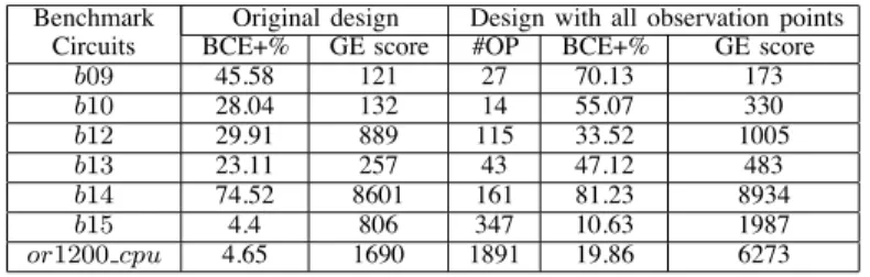
TABLE III. Gate-level BCE+ and GE score of the design before and after inserting all observation points.

Benchmark Original design Design with all observation points

Circuits BCE+% GE score #OP BCE+% GE score

b09 45.58 121 27 70.13 173

b10 28.04 132 14 55.07 330

b12 29.91 889 115 33.52 1005

b13 23.11 257 43 47.12 483

b14 74.52 8601 161 81.23 8934

b15 4.4 806 347 10.63 1987

or1200 cpu 4.65 1690 1891 19.86 6273

C. Maximum defect coverage for the design with all observation points inserted

The defect coverage of a functional test sequenceS is determined by the quality ofS, and the controllability and observability of the design. The defect coverage can be enhanced by improving the quality ofS or by inserting control and observation points to the design. We focus here only on selection and insertion of observation points so thatS can be made more effective for manufacturing test. Therefore, it is of interest to determine the maximum gate-level fault coverage when all possible observation points are inserted, and to normalize the fault coverage to this maximum when we evaluate the impact of inserting a subset of all possible observation points.

Tables II-III compare the stuck-at and transition fault coverage as well as two gate-level metrics (BCE+ and GE score) for the original design to the design with all observation points inserted. The parameters SFC% and TFC% represent stuck-at and transition fault coverage respectively. The parameterBCE+% indicates the gate-level fault coverage for bridging fault estimate. #OP lists the number of observation points. The or1200 cpu entry represents the CPU/DSP unit of the OpenRISC 1200 processor. Since we are focused on observation-point selection in this paper, we will consider the maximum gate-level fault coverage for the design with all observation points inserted as a measure of the highest achievable gate-level fault coverage. This maximum value is then used to normalize the fault coverage for the design with only a subset of observation points inserted.

D. Comparison of normalized gate-level fault coverage

In this section, we compare the normalized gate-level metrics (stuck-at fault coverage, transition fault coverage,BCE+ and GE score) for different observation-point selection methods. The normalized stuck-at fault coverage, transition fault coverage,BCE+ and GE score are obtained by taking the stuck-at fault coverage, transition fault coverage,BCE+ and GE score of the design with all observation points inserted as the reference.

An automatic method to select observation signals for design veriﬁcation was proposed in recent work [38]. Since this method is also applicable to observation-point selection in manufacturing test, we take it as an example of recent related work. For the sixIT C^′99

(5)

58 63 68 73 78 83 88 93 98

9 17 25 Number of observation points

Fault coverage

Original Proposed [32] Random

Case (1) BCE+

39 44 49 54 59 64 69 74 79 84 89 94

Normalized GE score

Case (2) GE score (a) b09

49 54 59 64 69 74 79 84 89 94 99

Fault coverage

Case (1) BCE+

34 39 44 49 54 59 64 69 74 79 84 89 94 99

Normalized GE score

Case (2) GE score (b) b10

88 89 90 91 92 93 94 95 96 97 98 99 100

Fault coverage

Case (1) BCE+

88 89 90 91 92 93 94 95 96 97 98 99 100

Normalized GE score

Case (2) GE score (c) b12 Fig. 3. Results on gate-level normalized metrics for b09, b10 and b12: (1) BCE+; (2) GE score.

37 42 47 52 57 62 67 72 77 82 87 92

Fault coverage

Case (1) BCE+

38 43 48 53 58 63 68 73 78 83 88 93

Normalized GE score

Case (2) GE score (a) b13

90 91 92 93 94 95

Fault coverage

Case (1) BCE+

94 95 96 97 98 99 100

Normalized GE score

Case (2) GE score (b) b14

34 39 44 49 54 59 64 69 74

Fault coverage

Case (1) BCE+

39 44 49 54 59 64 69 74 79 84

Normalized GE score

Case (2) GE score (c) b15 Fig. 4. Results on gate-level normalized metrics for b13, b14 and b15: (1) BCE+; (2) GE score.

(6)

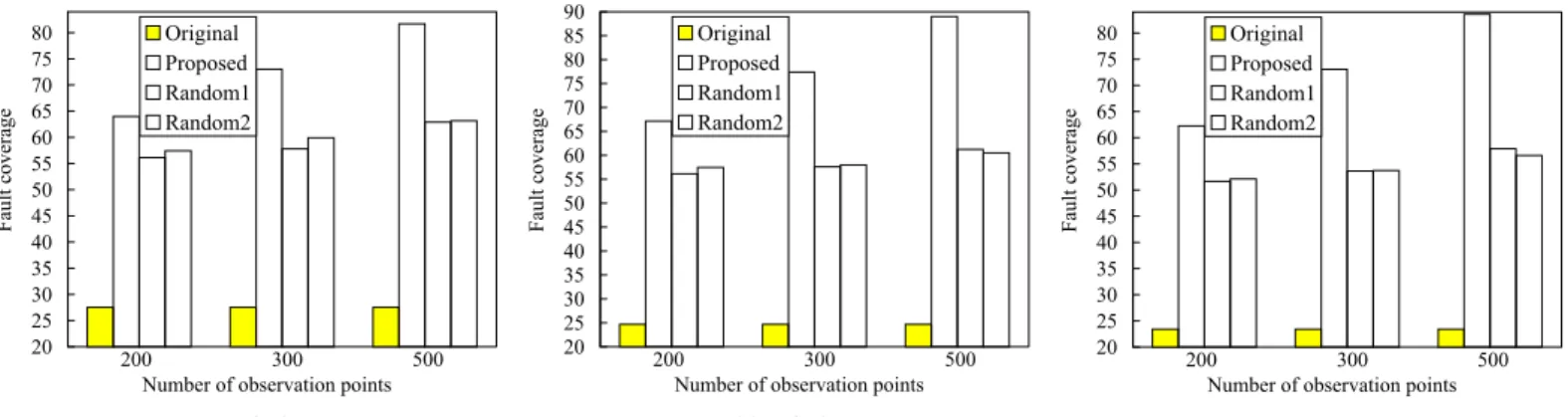
20 25 30 35 40 45 50 55 60 65 70 75 80

Fault coverage

Original Proposed Random1 Random2

Case (1) stuck-at fault coverage

20 25 30 35 40 45 50 55 60 65 70 75 80 85 90

Fault coverage

Case (2) transition fault coverage

20 25 30 35 40 45 50 55 60 65 70 75 80

Fault coverage

Case (3) BCE+ Fig. 5. Results on gate-level normalized metrics foror1200 cpu: (1) stuck-at fault coverage; (2) transition fault coverage; (3) BCE+.

circuits, we compare the proposed method to [38] and to a baseline random observation-point insertion method. For or1200 cpu, we compare the proposed method to two baseline random observation- point insertion methods since the method implemented by [38] is not directly applicable to it.

For each circuit, we select the same number ofn (for various values of n) observation points using different methods. Results for normalized gate-level fault coverage and normalized GE score are shown in Fig. 3-6. Due to lack of space, results for normalized gate-level stuck-at fault coverage and transition fault coverage for IT C^′99 circuits are on the web [39]. The results for all cases show that the proposed method consistently outperforms the baseline methods in terms of defect coverage metrics. Also, by inserting a small fraction of all possible observation points using the proposed method, signiﬁcant increase in defect coverage are obtained for all circuits. For each circuit, it only costs several seconds to calculate RT-level deviations and select observation points. These indicate the effectiveness of the proposed RT-level observation-point selection method.

E. Impact of functional coverage on the final defect coverage In this section, we will analyze the impact of functional coverage on the final defect coverage obtained for the design with all observation points inserted. One of the most commonly used functional coverage metric is the state coverage [40]–[42]. State is defined as the values of the state variables in the design. State coverage is defined as the ratio of the states covered by a test sequence over the target states. Here we consider the complete state set as the target states.

Table IV lists the state coverage for the sixIT C^′99 circuits.

“No. of Register Bits” represents the total number of bits for all state variables in the design. “Target States” lists the number of all possible states. “Covered States” shows the number of states covered by the given functional test sequences. The last column shows the state coverage. We can see that the state coverage is very low for each circuit.

In order to see the impact of state coverage on the ﬁnal defect coverage, we investigate the correlation between the state coverage and the gate-level fault coverage metric. Since the state coverage is quite low, we transform it by performing “log” operation on its denominator. For example, forb09, the state coverage is 390/2²⁸. We transform it to 390/log(2²⁸), that is 390/(28 ∗ log(2)). In this way, we can get the transformed format of state coverage for each circuit, denoted as a vector T rans state cov (T rans state cov b09, ..., T rans state cov b15). Next, we record the gate-level stuck-at fault coverage of the design

TABLE IV. State coverage.

Benchmark No. of Target Covered State

Register Bits States States Coverage

b09 28 ²²⁸ 390 ³⁹⁰/2²⁸

b10 20 ²²⁰ 160 ¹⁶⁰/2²⁰

b12 122 ²¹²² 1230 ¹²³⁰/2¹²²

b13 53 ²⁵³ 1141 ¹¹⁴¹/2⁵³

b14 216 ²²¹⁶ 4695 ⁴⁶⁹⁵/2²¹⁶

b15 417 ²⁴¹⁷ 117 ¹¹⁷/2⁴¹⁷

TABLE V. Kendall’s correlation coefﬁcient.

Stuck-at Transition BCE+ Fault Fault

Coefﬁcient 0.733 0.6000 0.6000

with all observation points inserted as a vector stuck cov (stuck cov b09, ..., stuck cov b15). Then, we calculate the Kendall’s correlation coefficient between T rans state cov and stuck cov. In the similar way, we calculate the Kendall’s correlation coefficient between the transformed form of state coverage and transition fault coverage (BCE+). Table V shows the correlation between transformed form of state coverage and stuck-at fault coverage (transition fault coverage,BCE+ metric). We see that the coefficients are significant. The results demonstrate that the higher transformed state coverage a design has, the more tendentious for the design with all observation points inserted to provide higher defect coverage.

IV. CONCLUSIONS

We have proposed an RT-level deviations metric and shown how it can used in combination with topology information to select and insert observation points for an RT-level design and a functional test sequence. This DFT approach allows us to increase the effectiveness of functional test sequences (derived for pre- silicon validation) for manufacturing testing. Experiments on six IT C^′99 benchmark circuits and the OpenRISC 1200 cpu show that the proposed RT-level DFT method outperforms two baseline methods for enhancing defect coverage (represented by stuck-at fault coverage, transition fault coverage, BCE+ and GE score). We have also shown that the RT-level deviations metric allows us to select a small set of the most effective observation points. As future work, we are applying the proposed method to the selection of control points to further increase the effectiveness of given functional test sequences.

REFERENCES

[1] M. L. Bushnell and V. D. Agrawal, Essentials of Electronic Testing. Kluwer Academic Publishers, Norwell, MA, 2000.

[2] J. Rearick and R. Rodgers, “Calibrating clock stretch during AC scan testing,” in Proc. ITC, 2005, pp. 266–273.

(7)

25 30 35 40 45 50 55 60 65 70 75 80 85 90 95

Normalized GE score

Fig. 6. Results on the gate-level normalized GE score metric foror1200 cpu. [3] J. Gatej et al., “Evaluating ATE features in terms of test escape rates and other

cost of test culprits,” in Proc. ITC, 2002, pp. 1040–1049.

[4] P. C. Maxwell, I. Hartanto, and L. Bentz, “Comparing functional and structural tests,” in Proc. ITC, 2000, pp. 400–407.

[5] A. K. Vij, “Good scan= good quality level? well, it depends...” in Proc. ITC, 2002, p. 1195.

[6] P. A. Thaker et al., “Register-transfer level fault modeling and test evaluation- techniques for VLSI circuits,” in Proc. ITC, 2000, pp. 940–949.

[7] F. Corno et al., “RT-level ITC’99 benchmarks and ﬁrst ATPG result,” IEEE Design & Test of Computers, vol. 17, pp. 44–53.

[8] M. B. Santos et al., “TL-based functional test generation for high defects coverage in digital systems,” Journal of Electronic Testing: Theory and Applications (JETTA), vol. 17, pp. 311–319.

[9] W. Mao and R. K. Gulati, “Improving gate level fault coverage by RTL fault grading,” in Proc. ITC, 1996, pp. 150–159.

[10] S. Ravi and N. K. Jha, “Fast test generation for circuits with RTL and gate- level views,” in Proc. ITC, 2001, pp. 1068–1077.

[11] I. Ghosh and M. Fujita, “Automatic test pattern generation for functional RTL circuits using assignment decision diagrams,” in Proc. Design Automation Conference, 1999, pp. 43–48.

[12] H. Kim and J. P. Hayes, “High-coverage ATPG for datapath circuits with unimplemented blocks,” in Proc. ITC, 1998, pp. 577–586.

[13] O. Goloubeva et al., “High-level and hierarchical test sequence generation,” in Proc. HLDVT, 2002, pp. 169–174.

[14] N. Yogi and V. D. Agrawal, “Spectral RTL test generation for gate-level stuck- at faults,” in Proc. Asian Test Symposium, 2006, pp. 83–88.

[15] T. Hosokawa, R. Inoue, and H. Fujiwara, “Fault-dependent/independent test generation methods for state observable FSMs,” in Proc. Asian Test Sympo- sium, 2007, pp. 275–280.

[16] R. Inoue, T. Hosokawa, and H. Fujiwara, “A test generation method for state- observable FSMs to increase defect coverage under the test length constraint,” in Proc. Asian Test Symposium, 2008, pp. 27–34.

[17] Y. Huang, C.-C. Tsai, N. Mukherjee, O. Samman, W.-T. Cheng, and S. M. Reddy, “Synthesis of scan chains for netlist descriptions at RT-level,” Journal of Electronic Testing: Theory and Applications (JETTA), vol. 18, pp. 189–201, 2002.

[18] C. Aktouf, H. Fleury, and C. Robach, “Inserting scan at the behavioral level,” IEEE Design and Test of Computers, vol. 17, pp. 34–42, 2000.

[19] S. Bhattacharya and S. Dey, “H-SCAN: A high level alternative to full-scan testing with reduced area and test application overheads,” in Proc. VTS, 1996, pp. 74–80.

[20] T. Asaka, S. Bhattacharya, S. Dey, and M. Yoshida, “H-SCAN+: A practical low-overhead RTL design-for-testability technique for industrial designs,” in Proc. ITC, 1997, pp. 265–274.

[21] S. Bhattacharya, F. Brglez, and S. Dey, “Transformations and resynthesis for testability of RT-level control-data path speciﬁcations,” IEEE Trans. VLSI Syst., vol. 1, pp. 304–318, 1993.

[22] S. Dey et al., “Non-scan design-for-testability of RT-level data paths,” in Proc. ICCAD, 1994, pp. 640–645.

[23] R. B. Norwood and E. J. McCluskey, “Orthogonal scan: Low overhead scan for data paths,” in Proc. ITC, 1996, pp. 659–668.

[24] I. Ghosh, A. Raghunathan, and N. K. Jha, “Design for hierarchical testability of RTL circuits obtained by behavioral synthesis,” in Proc. IEEE International Conference on Computer Design, 1995, pp. 173–179.

[25] ——, “A design for testability technique for RTL circuits using control/data ﬂow extraction,” IEEE Trans. CAD, vol. 17, pp. 706–723, 1998.

[26] H. Wada et al., “Design for strong testability of RTL data paths to provide complete fault efﬁciency,” in Proc. IEEE Int. Conf. VLSI Design, 2000, pp. 300–305.

[27] H. Fujiwara et al., “A nonscan design-for-testability method for register- transfer-level circuits to guarantee linear-depth time expansion models,” IEEE Trans. CAD, vol. 27, pp. 1535–1544, Nov. 2008.

[28] J. P. Grossman et al., “Hierarchical simulation-based veriﬁcation of Anton, a special-purpose parallel machine,” in Proc. IEEE International Conference on Computer Design, 2008, pp. 340–347.

[29] D. A. Mathaikutty et al., “Model-driven test generation for system level validation,” in Proc. HLDVT, 2007, pp. 83–90.

[30] O. Guzey and L.-C. Wang, “Coverage-directed test generation through auto- matic constraint extraction,” in Proc. HLDVT, 2007, pp. 151–158.

[31] H. Fang et al., “RT-level deviation-based grading of functional test sequences,” in Proc. VTS, 2009, pp. 264–269.

[32] http://www.opencores.org/openrisc,or1200.

[33] B. Benware et al., “Impact of multiple-detect test patterns on product quality,” in Proc. ITC, 2003, pp. 1031–1040.

[34] H. Tang et al., “Defect aware test patterns,” in Proc. DATE, 2005, pp. 450–455. [35] K. Y. Cho, S. Mitra, and E. J. McCluskey, “Gate exhaustive testing,” in Proc.

ITC, 2005, pp. 771–777.

[36] R. Guo et al., “Evaluation of test metrics: Stuck-at, bridge coverage estimate and gate exhaustive,” in Proc. VTS, 2006, pp. 66 – 71.

[37] B. J. Chalmers, Understanding Statistics. CRC Press, 1987.

[38] T. Lv, H. Li, and X. Li, “Automatic selection of internal observation signals for design veriﬁcation,” in Proc. VTS, 2009, pp. 203–208.

[39] http://people.ee.duke.edu/∼hf12/.

[40] R. Taylor, D. Levine, and C. Kelly, “Structural testing of concurrent programs,” IEEE Transactions on Software Engineering, vol. 18, pp. 206–215, 1992. [41] J. Carletta and C. Papachristou, “A method for testability analysis and BIST

insertion at the RTL,” in Proc. European Design and Test Conference, 1995, p. 600.

[42] S. Gupta, J. Rajski, and J. Tyszer, “Arithmetic additive generators of pseudo- exhaustive test patterns,” IEEE Transactions on Computers, vol. 45, pp. 939– 949, 1996.

C209 2009 11 WRTLT 最近の更新履歴 Hideo Fujiwara

Observation-Point Selection at the Register-Transfer Level to

Enhance Defect Coverage for Functional Test Sequences ∗

Enhance Defect Coverage for Functional Test Sequences ^∗