MATLAB PRIMER
Multi dimensional array in MATLAB
June, 8th, 2015 Hiroyuki AKAMA
Data formats
Scalar: 0 dimensional array, "null-dimensional" matrix, i.e. only one element Vector : One-dimensional matrix
Matrix: Array with more than two dimensions.
Square brackets [] represent Scalar, Vector, or Matrix.
Scalar
>> sc =64 sc = 64
>> sc=64; % A semi-colon mark ; suppress the display of an answer. A percent mark % is for setting a comment line.
>> sc2=[64] sc2 = 64
>> sc(1,1) %a scalar is considered as a one-by-one matrix. ans =
64
>> sc2(1,1) ans = 64
>> sc==sc2 %Regardless of the presence of [], scalar would be indifferent, so that this command returns1, which means true.
ans = 1
>> isscalar(sc) %logically true. ans =
1
>> isscalar(sc2) ans =
1
>> size(sc) %Even for a scalar, it size has two dimmensions. ans =
1 1
>> size(sc2) ans =
1 1
Vector
>> rvect = [2 5 6]; %A row vector with three elements. The separator is a space. rvect = [2,5,6]; %A comma ',' can be also used as a separator.
rvect(2) %The second element of this vector. rvect(0) %There is no 0th element in Matlab. ans =
5
??? 添字 インデックス 実数 正 整数 論理値 い れ でなけれ なりま ん
>> cvect = [14; 86; inf] %A column vector. A semi-colon ';' is use for separating columns.
cvect(1:2) %The first and second elements are extracted from the vector. seq = 0:2:10 %A sequence of integers from 0 through ten with a step of two. seq2 = 10:15
seq2' %An apostrophe ''' means transposition.
seq2'==transpose(seq2) %identical to the function of transpose() cvect =
14 86 Inf ans = 14 86 seq =
0 2 4 6 8 10
seq2 =
10 11 12 13 14 15
ans = 10
11
12
13
14
15
ans = 1
1
1
1
1
1
>> size(seq2) ans = 1 6
>> size(seq2') ans = 6 1
Matrix >> mat1=[1 5 2;3 9 7;8 6 2] %A three by three matrix. mat1 = 1 5 2
3 9 7
8 6 2
>> mat1(2) %The indexing is made by vertically counting the positions of elements from top to bottom. ans = 3
>> mat1(4) %The forth element (with the index of 4) is 5 in the cell position of (1,2). ans =
5
>> mat1(2,:)%A colon mark ':' represents all so that in this case all the elements in the 2nd column are enumerated.
ans =
3 9 7
>> mat1(:,3)%The 3rd column is extracted. ans =
2 7 2
>> mat1(2:3,1:2)%The sub matrix (the 2nd to third rows and the first to second columns ) is taken.
ans =
3 9 8 6
>> mat1(2,3) %The element in the cell of (2,3). ans =
7
>> mat1(8) %The 8th element. Identical to the previous command. ans =
7
>> sub2ind(size(mat1),2,3)% The function of 'sub2ind' converts subscripts to linear indices. What is the serial number of the position of second in row and third in column for any matrix of which the size is identical to that of mat1?
ans = 8
>> [p,q]=ind2sub(size(mat1),8)%The function of 'index2sub' allows us to get subscripts from linear index. What is the position of 8 in serial index for mat1? the position number is given as the second argument.
%As there are two returned values, so an array with two slots should be set on the left hand.
p = 2 q = 3
>>invmat1=inv(mat1); %inv() gives the inverse matrix of mat1.
>> round(invmat1*mat1)% This function does rounding of a real number to the nearest integer.
ans =
1 0 0 0 1 0 0 0 1
>> eye(3) %Identity matrix ans =
1 0 0 0 1 0 0 0 1
>> round(invmat1*mat1)==eye(3) %All true. ans =
1 1 1 1 1 1 1 1 1
II. Random number
rand():This function provides an array of rand values following the uniform distribution.
%r = rand(n) returns an n-by-n square random matrix of which the values are provided according to the uniform distribution on the open interval of (0,1).
%r = rand(m,n) or r = randn([m,n]) returns an m-by-n random matrix.
>> rand(3) ans =
0.4218 0.9595 0.8491 0.9157 0.6557 0.9340 0.7922 0.0357 0.6787
>> rand([3 4]) ans =
0.6324 0.5469 0.1576 0.4854 0.0975 0.9575 0.9706 0.8003
0.2785 0.9649 0.9572 0.1419
randn():creates a matrix of pseudo-random values following the normal distribution.
>> randn(2) ans =
0.5377 -2.2588 1.8339 0.8622
>> randn([3 4]) ans =
1.0347 0.2939 -1.1471 -2.9443 0.7269 -0.7873 -1.0689 1.4384 -0.3034 0.8884 -0.8095 0.3252
normrnd(): Requires Statistics ToolBox.
%normrnd(mu,sigma) generates random numbers from the normal distribution with mean parameter mu and standard deviation parameter sigma
normrnd(0,1)
random(): Requires Statistics ToolBox 必要
% random(stats) provides a random value following the distribution specified as the 2st argument.
%The following returns a three by five random array following the standard normal distribution(mean: 0; standard deviation 1).
random('Normal',0,1,3,5)
randomsample():Requires Statistics ToolBox.
%randsample(n,k) returns a k-by-1 vector of integers extracted from 1 to n through a random sampling without replacement.
Advanced Topics
I. Initialization for running a for loop. It is to better to reserve a set of memory corresponding to the shape of the output (array to be created) using zeros() command. You can initialize an empty array but from the viewpoint of computational speed, it is not a good solution.
Revise the following program by initially setting a zero array with a fixed size using the function of zeros(). A multidimensional array with the size of 40-by-5-by-7 will be created at the end.
Program 1A
repetitionTime=40;
myarray=[]; %An empty array for i=1:repetitionTime
myarray= [myarray;rand(1,5,7)];
%Pay attention to the semicolon mark(";") in the array. %What will be produced if removing this semi-colon? end
myarray size(myarray)
Program1B:
repetitionTime=40;
myarray=zeros(repetitionTime,5,7); for i=1:repetitionTime
myarray(i,:,:)= rand(1,5,7); end
myarray size(myarray)
program2A:
repetitionTime=40;
myarray=[]; %An empty array for i=1:repetitionTime
myarray= [myarray rand(1,5,7)];
end myarray size(myarray)
%1 200 7
Program2B:
repetitionTime=40;
myarray=zeros(1,5*repetitionTime,7);; %An empty array
????????
myarray size(myarray)
%1 200 7
Exercise
1) Create a 10 by 10 square random array in which all the values follow the uniform distribution between 0 and 1 and save the result in the variable randmatrix.
2) randmatrix(4,5)== randmatrix(one_integer) returns 1.
What is a value of one_integer?
3) one_integer ==one_function(size(randmatrix),4,5) returns 1.
What is the name of the function one_function?
Simulation and visualization in Matlab (This file is under construction)
June, 15th, 2015 Hiroyuki AKAMA
Review
>> p=[1 2 3;4 5 6;7 8 9] % A 2D array (matrix) with the size of 3-by-3 is defined, The %
mark is to put a comment line.
p =
1 2 3 4 5 6 7 8 9
>> tp=p' %transposition. You can run also transpose(p) instead.
tp =
1 4 7 2 5 8 3 6 9
>> size(p) %The length of an array is computed according to the dimensionality.
ans =
3 3
>> tp(1) %The serial order is set along the direction of columns (from top to bottom before moving on to the next column)
ans =
1
>> tp(2)
ans =
2
>> tp(3)
ans =
3
>> tp(4)
ans =
4
>> tp(1,:) % A colon mark represents all the columns here.
ans =
1 4 7
>> tp(:,1)
ans =
1 2 3
>> tp(2,3) %the element at the 2nd row and the third column is extracted.
ans =
8
>> p+tp
ans =
2 6 10 6 10 14 10 14 18
>> p+tp==(p+tp)' %p+tp is symmetrical. Matlab returns 1 for TRUE evaluating all the corresponding elements in the two arrays.
ans =
1 1 1 1 1 1 1 1 1
>> p(:,:,2)=tp % How to create a 3-dimmensional array. A 3rd dimension is added to p.randi(9,9)
p(:,:,1) =
1 2 3 4 5 6 7 8 9
p(:,:,2) =
1 4 7 2 5 8 3 6 9
>> size(p)
ans =
3 3 2
A digital image is in reality an array of discrete values in each element
position (such as pixel).
A brain image scanned by an fMRI scanner is a three-dimensional array, which is composed of a set of triplets (x,y,z) as coordinate values.
A smallest data unit (atom) of brain image is called VOXEL, which means pixel with volume or thickness (with the direction of z-axis).
A voxel can be conceived as a rectangular cuboid in a 3D brain image.
When capturing a series of brain images in succession with a fixed interval of time called repetition time (TR) or volume time, an fMRI dataset takes a shape of 4 dimensions (4D).
You know: Matlab is good at matrices and vectors, and multi-dimensional arrays.
fMRI scanner Brain scans Voxel space: 3D array
Example of a 3D array
>> dummydata=rand(6,4,5)
dummydata(:,:,1) =
0.8147 0.2785 0.9572 0.7922 0.9058 0.5469 0.4854 0.9595 0.1270 0.9575 0.8003 0.6557 0.9134 0.9649 0.1419 0.0357 0.6324 0.1576 0.4218 0.8491 0.0975 0.9706 0.9157 0.9340
dummydata(:,:,2) =
0.6787 0.7060 0.6948 0.7655 0.7577 0.0318 0.3171 0.7952 0.7431 0.2769 0.9502 0.1869 0.3922 0.0462 0.0344 0.4898 0.6555 0.0971 0.4387 0.4456 0.1712 0.8235 0.3816 0.6463
dummydata(:,:,3) =
0.7094 0.1190 0.7513 0.5472 0.7547 0.4984 0.2551 0.1386 0.2760 0.9597 0.5060 0.1493 0.6797 0.3404 0.6991 0.2575 0.6551 0.5853 0.8909 0.8407 0.1626 0.2238 0.9593 0.2543
dummydata(:,:,4) =
0.8143 0.6160 0.9172 0.0759 0.2435 0.4733 0.2858 0.0540 0.9293 0.3517 0.7572 0.5308 0.3500 0.8308 0.7537 0.7792 0.1966 0.5853 0.3804 0.9340 0.2511 0.5497 0.5678 0.1299
dummydata(:,:,5) =
0.5688 0.3112 0.6892 0.1524 0.4694 0.5285 0.7482 0.8258 0.0119 0.1656 0.4505 0.5383 0.3371 0.6020 0.0838 0.9961 0.1622 0.2630 0.2290 0.0782
0.7943 0.6541 0.9133 0.4427
%Using a function for generating a set of random numbers following a certain statistical distribution is an important step for executing simulation. Note that creating random numbers means setting a population under a null hypothesis.
%Ans (Answer) here is displayed as an ordered series of two dimensional matrices of which the number is that the third argument as z for the function rand() to create a random 3D array. En each matrix, all the x and y values are enumerated so the expression is made with two colons such as dummydata(:,:,<z value>).
>>imagesc(dummydata(:,:,1))
This map created by the function of imagesc(matrix) represents the matrix of dummydata(:,:,1) as the first x-y slice. The plane depicted here is a sort of heat map in which each real number corresponds to each color according to a color scale. The smaller the value is the more bluish the corresponding square becomes. Inversely, the larger the value is the more reddish the corresponding square becomes. This example can be considered as a basic example for how a brain scan is displayed from a digital 3D array dataset.
>>imagesc(dummydata(:,:,2))
%The second x-y (axial) slice.
Attention!
>>imagesc(dummydata(:,1,:)) does not work!
We run the following command to get a set of x-z (coronal) slices from this dummy
dataset.
>>permute(dummydata,[1 3 2])
The function of permute(array, order) allows us to transpose the array given as the first argument following the order specified as an array for the second argument.
So we might want to execute
>>permdata= permute(dummydata,[1 3 2]);
>>imagesc(permdata(:,:,1))
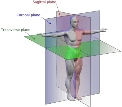
Q. How do you have to do in order to get a y-z (saggittal) slice ?
Figure replicated from Wikipedia
How to save the image files for all the axial (x-y) slices of this dataset. First of all, we should make sure the size of this dataset.
>> size(dummydata)
ans =
6 4 5
>> size(dummydata,3)
ans =
5
%Let’s suppose 'C:¥Users¥akama-h-aa¥¥axial_slice’ is the directory in which you save your picture files. It depends on your own environement.
for i = 1 : size(dummydata,3)
saveas(imagesc(p(:,:,i)), strcat('C:¥Users¥akama-h-aa¥¥axial_slice_', num2str(i), '.jpg'),'jpg');
end
% You ran a ‘for’ loop to repeatedly perform the same work for each slice by incrementing the slice number. The function of strcat() is to concatenate multiple character strings. The function of num2str() is used to convert a number to the corresponding character.
4D array
The command of rand() can take the arbitrary number of arguments. Here is an instance of a random 4D tansor.
>> rand(5,3,4,2)
ans(:,:,1,1) =
0.1067 0.8687 0.4314 0.9619 0.0844 0.9106 0.0046 0.3998 0.1818 0.7749 0.2599 0.2638 0.8173 0.8001 0.1455
ans(:,:,2,1) =
0.1361 0.8530 0.0760 0.8693 0.6221 0.2399 0.5797 0.3510 0.1233
0.5499 0.5132 0.1839 0.1450 0.4018 0.2400
ans(:,:,3,1) =
0.4173 0.4893 0.7803 0.0497 0.3377 0.3897 0.9027 0.9001 0.2417 0.9448 0.3692 0.4039 0.4909 0.1112 0.0965
ans(:,:,4,1) =
0.1320 0.2348 0.1690 0.9421 0.3532 0.6491 0.9561 0.8212 0.7317 0.5752 0.0154 0.6477 0.0598 0.0430 0.4509
ans(:,:,1,2) =
0.5470 0.1835 0.9294 0.2963 0.3685 0.7757 0.7447 0.6256 0.4868 0.1890 0.7802 0.4359 0.6868 0.0811 0.4468
ans(:,:,2,2) =
0.3063 0.6443 0.9390 0.5085 0.3786 0.8759 0.5108 0.8116 0.5502
0.8176 0.5328 0.6225 0.7948 0.3507 0.5870
ans(:,:,3,2) =
0.2077 0.1948 0.3111 0.3012 0.2259 0.9234 0.4709 0.1707 0.4302 0.2305 0.2277 0.1848 0.8443 0.4357 0.9049
ans(:,:,4,2) =
0.9797 0.5949 0.1174 0.4389 0.2622 0.2967 0.1111 0.6028 0.3188 0.2581 0.7112 0.4242 0.4087 0.2217 0.5079
Now let’s try to think about how to add to the original 3D array (representing a brain scan) another one recorded at another time point in the same experiment session to make a 4D dataset.
Given a 3D array p, the 4th dimension (=time) is added as follows.
p(:,:,1,1) is the image of the slice 1 at the time point 1; p(:,:,1,2) is the image of the slice 1 at the time point 2; p(:,:,2,1) is the image of the slice 2 at the time point 1; p(:,:,2,2) is the image of the slice 2 at the time point 2.
>> n = 3; %number of time points. for i = 1 : size(dummydata,3) for j = 1 : n
if j == 1
newscan=dummydata; else
newscan=rand(6,4,5); end
dummydata(:,:,i,j)=newscan(:,:,i); end
end
%We used a double for loop. The outside for loop was run to exhaustively take the x-y slices at each time point. We have n time point. Note that we need to close each block for condition control by an end. Pay attention to the indent at every line.
>> size(dummydata) %The fourth dimension has been added.
ans =
6 4 5 3
>> dummydata(:,:,:,1)
% same as the previous dummydata ans(:,:,1) =
0.8147 0.2785 0.9572 0.7922 0.9058 0.5469 0.4854 0.9595 0.1270 0.9575 0.8003 0.6557 0.9134 0.9649 0.1419 0.0357 0.6324 0.1576 0.4218 0.8491 0.0975 0.9706 0.9157 0.9340
ans(:,:,2) =
0.6787 0.7060 0.6948 0.7655 0.7577 0.0318 0.3171 0.7952 0.7431 0.2769 0.9502 0.1869 0.3922 0.0462 0.0344 0.4898 0.6555 0.0971 0.4387 0.4456 0.1712 0.8235 0.3816 0.6463
ans(:,:,3) =
0.7094 0.1190 0.7513 0.5472 0.7547 0.4984 0.2551 0.1386 0.2760 0.9597 0.5060 0.1493 0.6797 0.3404 0.6991 0.2575 0.6551 0.5853 0.8909 0.8407 0.1626 0.2238 0.9593 0.2543
ans(:,:,4) =
0.8143 0.6160 0.9172 0.0759 0.2435 0.4733 0.2858 0.0540 0.9293 0.3517 0.7572 0.5308 0.3500 0.8308 0.7537 0.7792 0.1966 0.5853 0.3804 0.9340 0.2511 0.5497 0.5678 0.1299
ans(:,:,5) =
0.5688 0.3112 0.6892 0.1524 0.4694 0.5285 0.7482 0.8258 0.0119 0.1656 0.4505 0.5383 0.3371 0.6020 0.0838 0.9961 0.1622 0.2630 0.2290 0.0782 0.7943 0.6541 0.9133 0.4427
>> permute(permdata,[1 3 2])==dummydata(:,:,:,1)
%Make sure that the original dummydata, which can be restored as permute(permdata,[1 3 2]) is now identical to dummydata(:,:,:,1).
ans(:,:,1) =
1 1 1 1
1 1 1 1
1 1 1 1
1 1 1 1
1 1 1 1
1 1 1 1
ans(:,:,2) = 1 1 1 1
1 1 1 1
1 1 1 1
1 1 1 1
1 1 1 1
1 1 1 1
ans(:,:,3) = 1 1 1 1
1 1 1 1
1 1 1 1
1 1 1 1
1 1 1 1
1 1 1 1
ans(:,:,4) = 1 1 1 1
1 1 1 1
1 1 1 1
1 1 1 1
1 1 1 1
1 1 1 1
ans(:,:,5) =
1 1 1 1
1 1 1 1
1 1 1 1
1 1 1 1
1 1 1 1
1 1 1 1
The following is a command to save all the variable data on the memory (appearing in the workspace) in a single mat file (file extension: mat), binary file specific to Matlab.
>> save('Matlab-course-09.mat')
You can reload this file next time by running
>>load('Matlab-course-09.mat')